1. Introduction

The present work is concerned with flow control of aerodynamic or hydrodynamic surfaces, in particular with passive flow control devices. The motivation of such surfaces with respect to passive flow control may give potential gains in terms of hydrodynamic and aerodynamic performance for engineering designs such as aircraft wings, control surfaces, propellers, fans, wind turbines, and automotive airfoils [¹].

In some cases, studies may find inspiration by simply observing how Nature works. In that sense, the observation of humpback whales flipper patterns brought to light an interest in the wavy leading edge phenomena.Despite its large size, the humpback whale is agile when it is maneuvering and swimming with its flippers at high angles of attack. With this in mind, [²] suggested that the presence of tubercles (wavy leading edge) on the flippers plays an essential role on the maneuvering capability of the humpback whales, in particular when they are feeding.

Motivated by the tubercles function of the humpback flipper, [³] carried out numerical studies of the sinusoidal leading edge that showed a potential gain in aerodynamic and hydrodynamic efficiency. These simulations were performed using an airfoil NACA 63021 with finite-span (aspect ratio of 2.04). The panel method with an inviscid flow suitable for large Reynolds number was employed. At an angle of attack 10 degrees, the wavy shape incorporated at the leading edge resulted in an increase of 4.8% in the lift force, a decrease of 10.9% in the induced drag, and an increase in the lift to drag ratio by 17.6%. With the work of [³], it may be concluded that the wavy leading edge enhances wing performance at modest angles of attack, while offering no significant effects at zero angles of attack. However, for a viscous calculation form drag increases by 11% at α = 10◦.

The first experimental study of the wavy leading edge was carried out by [⁴], who built a scale model of a flipper using a NACA 0020 airfoil in wind tunnel testing with a Reynolds number range from 505,000 to 520,000. The tests showed promising results with an increase of 40% on the stall angle and 6% in the maximum lift, and a decrease of 32% in the drag on the post-stall regime when compared with smooth flipper model. At a low angle of attack, both models showed similar results. However, at a limited range of 10.3 ^◦ < α < 10.8 ^◦ , a higher drag was observed when compared with the correspond smooth model. The authors have observed that specifically the scalloped leading edge of flipper has the function of delaying stall, which provides higher lift at higher angles of attack. The results of [⁴] have motivated later studies in the wavy leading edge phenomenon [⁵-⁹].

There are many potential applications for wavy leading edge, especially at low Reynolds numbers regime. One of those is for UAVs (Unmanned aerial vehicle). That kind of aircraft has small chord length and fly at a relatively low speed, which means operating in low Reynolds number regime, such as a range of Reynolds number from 103 up to 8x10⁵ [¹⁰]. The maximum lift coefficient may decrease due the lower Reynolds number as within this regime the flow is more prone to flow separation. As a result, for an example of an aircraft, its performance may degenerate during landing or take-off. Studies presented in [¹¹] indicate that the use of tubercles allows a decrease of the minimum stall-speed without an increase of drag. In addition, within the low Reynolds number regime with wavy leading edge airfoils, it is worth mentioning other references such as De Paula [¹²-¹⁴] that presented an extensive experimental study, with applications to boat rudders, missile fins, and aircraft control surfaces.

Furthermore, helicopter and wind turbine blades could also benefit from wavy leading edge incorporation. Those often operate at high angles of attack and therefore subject to dynamic stall, these shapes could have smooth stall behavior, and consequently reduced fatigue with the addition of tubercles [¹⁵].

[¹⁶] conducted numerical simulation of flow around a NACA 63021 airfoil with tubercles at the leading edge. The results show that the tubercles generate vortex in the troughs in the chord-wise direction, which increase the velocity downstream of the tubercle peak. Locally, the flow resistance to adverse pressure gradient was increased. However, at the troughs region, the flow separation has been anticipated. As such, this work has also contributed to highlight the concept of moment exchange between peaks and troughs of the airfoil as a flow control mechanism of vortex generation.

Another numerical study at Reynolds number of 800 was conducted by [¹⁷]. This simulation shows that vortexes originate from both sides of the tubercles peaks in a counter-rotating manner, which form a Kelvin-Helmholtz instability. The Refs. [¹⁸] and [¹⁹] observed a similar behavior from their numerical simulation of an airfoil with tubercles at a higher Reynolds number of 120,000. Those studies use a stalled NACA 0021 airfoil at 20 degrees incidence angle making use of LES (Large Eddy Simulation) to resolve the flow. They also observed the Kelvin-Helmholtz instabilities at the peaks surfaces of the tubercles. The Ref. [¹⁸] noted another flow mechanism of airfoil with tubercles, in which a strong pressure gradient in the spanwise direction causes a secondary flow for a configuration with a wavy leading edge. This secondary flow contributes to boundary layer re-energizing, which delays flow separation.

Bolzon [²⁰] suggested that there is also a potential benefit of the application for high Mach number. In this case, one would be able to reduce the wave drag by the use of wavy leading edge.

In this context, for this work, several numerical simulations have been carried out to resolve the flow around an airfoil based on the NACA 0021 profile without and with wavy leading edge. The amplitude is 3% and the wavelength 11% both with respect to the airfoil chord, all simulations considered a high Reynolds number of 3X10⁶, which is based on the airfoil chord. Values of aerodynamic force coefficients as well as flow topology are presented for both cases without and with wavy leading edge. The obtained numerical results are analysed and compared to especially highlight advantages of the wavy leading configuration as well as its flow mechanism. The commercial CFD code, ANSYS FLUENT, has been employed for all simulations carried out in this work.

2. Theoretical formulation

The numerical method applied to resolve the flow is based on the finite volume method [21]. In addition, to deal with the high turbulent flow, the RANS equations are employed. The unknown Reynolds stress tensor of the RANS equations is resolved by applying turbulence modeling [21]. In this section, the formulation of the Reynolds Averaged Navier-Stokes (RANS) equations and of two turbulence models (k-ϵ and Spalart-Allmaras) are presented.

2.1 RANS equations

The equations of motion for RANS (Reynolds Averaged Navier-Stokes) is obtained by applying a time average of the Navier-Stokes equations with its flow variables decomposed by what is known as Reynolds decomposition [²²], i.e., the flow variables are decomposed into a time-averaged component, identified with an upper bar, and a time fluctuating component, identified with a prime mark. Finally, the RANS equations can be written for incompressible flows, as [²²] (1) and (2):

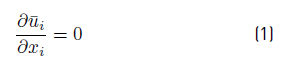
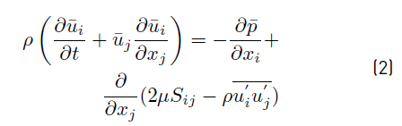
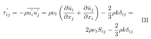
where ρ is the fluid density, μ denotes the fluid dynamic viscosity, p is the static pressure, ui represents the i-direction flow velocity vector component. The term ρu _i u _j is the Reynolds stress tensor and is initially unknown. Assuming Boussinesq’s hypothesis [²²], in which the Reynolds stress tensor (τ _ij ) is proportional to strain-rate tensor (S _ij ) (3):

Here 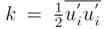is the turbulent kinetic energy per unit mass and ν _t is the eddy kinematic viscosity, also known as turbulent kinematic viscosity. From Equation (3), in order to close the RANS equations, the eddy kinematic viscosity should be resolved, as such, turbulence modeling may be applied.

2.2 Turbulence closure

For the closure of the RANS equations [²¹], two turbulence models k − ϵ and Spalart-Allmaras are considered in this work. The model k-ϵ, proposed by [²³, ²⁴], consists in the use of the conservation equations for the turbulent kinetic energy (k) and its dissipation (ϵ), which are both related to the eddy viscosity as (4) and (5):

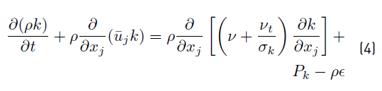
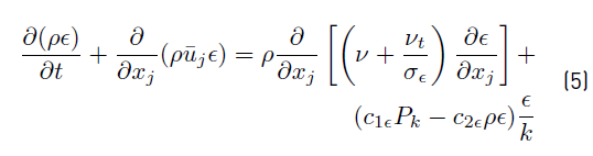
where the turbulent kinematic viscosity (ν _t ) is related to the turbulent quantities, k and ϵ, as (6):

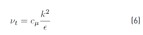
In these equations, c _μ , σ _k , σ _ϵ , c _1ϵ and c _2ϵ are constants. σ _k and σ _ϵ are Prandtl numbers connecting the diffusivity of k and ϵ to the eddy viscosity ν _t . All values are provided in [²¹].

The Spalart-Allmaras model consists of one transport equation based on the kinematic eddy viscosity parameter as proposed in [25]. The transport equation for is as follows (7):

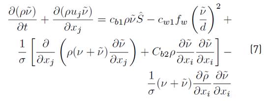
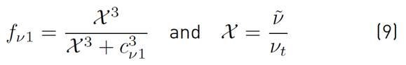
The turbulent eddy viscosity coefficient is obtained from (8):

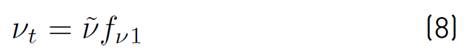
where f _ν1 is a wall-damping function, which tends to unity further from the wall, and zero towards the wall as (9):

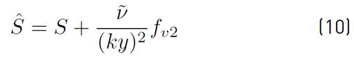
In Equation (7), the rate of production of is related to the local mean vorticity as follows (10):

where (11):

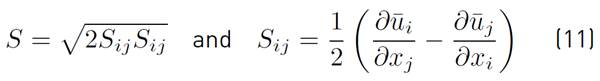
The functions fv2 and fw are other wall-damping functions, which are described in reference [25]. In addition, in the above equations of the model, c _ν1 , c _b1 , c _w1 and c _b2 are constants, whose values are given in reference [²⁵]

3. Numerical methodology, geometry and mesh

The discretization of the equations set presented above is performed using the finite volume method, according to the numerical methodology implemented in the ANSYS Fluent commercial code. Due to the low Mach number of the flow (Mach number of 0.269), the simulations are carried out with the flow considered as incompressible. As such, for incompressible flows, to deal with the pressure-velocity coupling, the SIMPLE (Semi-Implicit Method for Pressure Linked Equations) algorithm [²¹] is employed. For computing the gradients, the least-squares cell-based method is used. For all set of algebraic equations obtained from the discretization of the governing flow equations, the second-order upwind spatial discretization method is applied.

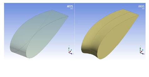
The two geometries of the airfoil, respectively, without and with wavy leading edge used for the numerical simulations are illustrated in Figure 1.

Figure 1 Airfoil geometry: straight leading edge (left) and wavy leading edge (right) 

3.1 Computational domain and boundary conditions

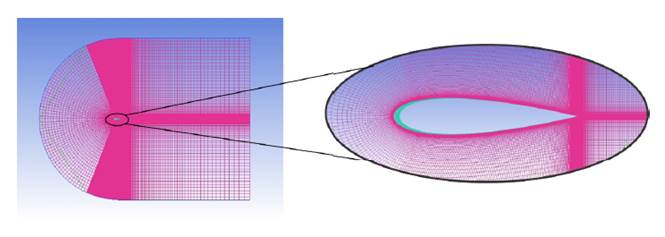
For the simulations, a computational domain was set surrounding the airfoil geometry with a C-type structured mesh as shown in Figure 2. The distance from the airfoil surface to the far-field boundaries is 12.5 times the airfoil chord. Along the spanwise direction, the distance used corresponds to the span of the airfoil of 11% of the airfoil chord. With respect to the boundary conditions applied. Uniform velocity is set at the inlet (Mach number of 0.269), with zero freestream turbulence. The boundaries at the bottom and top of the computational domain are set up as slip walls. At the outlet, the standard atmosphere pressure condition is employed, whereas periodicity is applied in the spanwise direction, that is, at the lateral boundaries. A nonslip wall condition is set up for the wing surface. No special treatment is required at the wall, since the grid is sufficiently fine to fully resolve the boundary layer, as y ⁺ ≈ 1.

With regard to the mesh, towards the wall surfaces the mesh is refined smoothly up to a non-dimensional wall distance of y+ ≈ 1. At the wake region, downstream the airfoil, the mesh is also smoothly refined, as shown in Figure 2. The mesh has a total of 2,288,000 cells. Along the spanwise direction 20 cell volumes are used, at the airfoil leading edge 230 cells volumes are applied, along the airfoil upper or botton surface 230 cells volumes are set and, finally, at the trailing edge 130 cells are used.

Figure 2 Computational mesh, medium refinement mesh 

4. Mesh sensitivity and prelimary simulations

Keeping the C-type structured mesh set-up as shown in Figure 2, three differentt levels of mesh refinement are considered to evaluate its influence on the numerical results, respectively, of 1,420,000 cells (coarse mesh), 2,288,000 cells (medium mesh) and 3,104,000 (fine mesh) cells. For the coarse and fine mesh, the same cell volume proportion number of the medium mesh as described in the previous section, is applied, which is, thus, scaled, respectively, to 1,420,000 and 3,104,000 cells.

For the numerical simulations, the following flow conditions were used: Reynolds number 3X10⁶, Mach number 0.269, temperature 298 K, reference pressure 101325 Pa, density 1.185 kg/m³, and the fluid viscosity of 1.836X10 ⁻⁵ kg/m.s. Due to the low Mach number of the flow of 0.269, the simulations are carried out considering the flow as incompressible.

In order to check the mesh refinement sensitivity to the numerical simulation, for a straight leading edge airfoil, the lift coefficient curves were obtained for the three meshes (coarse, medium and fine) considered as shown in Figure 3. The obtained lift curves are also compared with the corresponding data provided by the Xfoil panel method code [²⁶], and with the experimental data of [²⁷]. In Figure 3, the lift curve slopes within the linear behavior regime are all with a similar tendency, keeping this behaviour up to approximately an angle of attack of 12.5 ^◦ , just before the pre-stall regime, when viscous flow effects become more significant. For higher angles of attack, considering the maximum lift coefficient values, all cases considered, except for the experimental data, are in very good agreement, not exceeding a difference of 3%. In addition, the euclidean norm values of the lift coefficient for the three meshes are compared as shown in Figure 4. It can be noted that as the mesh is more refined, the change of the lift coefficient norm value decreases, as such, indicating a good convergence tendency as mesh is even more refined. Besides that, despite the difference of the lift coefficient norm values, the discrepancy between the coarse and fine mesh does not exceed 2%. Therefore, considering the good agreement of the results presented in Figures 3 and 4 for the three different meshes, the medium size mesh (as presented in Figure 2] is chosen as the standard mesh for all simulations to be presented for both with straight and wavy leading edge cases.

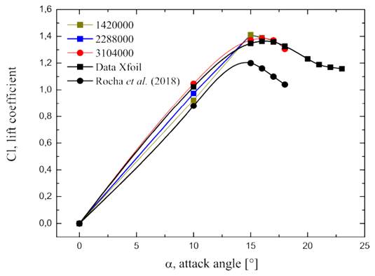
Figure 3 Lift curve for the three meshes considered being compared with data from Xfoil code and experimental result of [²⁷] 

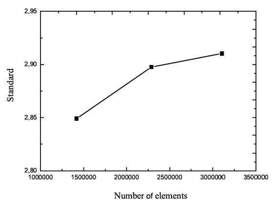
Figure 4 Euclidean norm values of the lift coefficient (denoted as standard) for the three meshes considered 

4.1 Turbulence modeling comparison and verification

Due to the high turbulent flow, the RANS equations are used as aforementioned, in which two different turbulence models are initially considered, respectively, the k-ϵ and Spalart-Allmaras models.

The aerodynamic lift forces for the straight leading edge configuration obtained by the two turbulent models are compared within the angle of attack range 0◦ < α < 22.5◦, for a Reynolds number of 3X106, as shown in Figure 5. The results are also compared with the corresponding experimental data extracted from [²⁷] and the Xfoil panel method code [²⁶]. From this study, it can be noted that the results provided by the Spalart-Allmaras turbulence model present better agreement with the corresponding results of Xfoil and [²⁷], especially at the post-stall regime. Thus, the Spalart-Allmaras turbulence model is chosen as the base RANS turbulence model for all numerical results to be presented with both straight and wavy leading edge configurations.

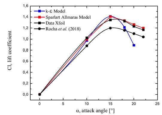
Figure 5 Lift coefficient curve against angle of attack obtained with the k − ϵ and Spalart-Allmaras turbulence models. Data are compared with Xfoil panel method code and experimental results of [²⁷] 

5. Results and discusión

The flow behaviour for the case with WLE (Wavy Leading Edge) is presented in this section by means of pressure and vorticity fields as well as wall shear stress, lift and drag forces and, finally, pressure coefficients on the airfoil surface. As aforementioned, all simulations were carried out for a Reynolds number of 3X10⁶ considering the Spalart-Allmaras turbulence model.

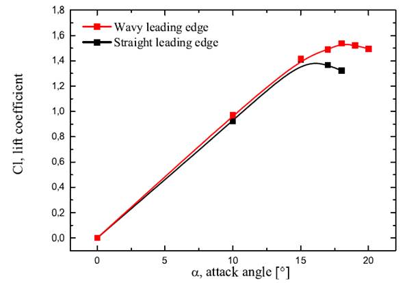
At first, the obtained lift curve behavior is presented in Figure 6, considering both cases with straight and wave leading edge configurations. The results show a similar lift curve slope for both configurations when the lift curve has a linear behaviour with respect to the angle of attack. However, when the lift curve slope starts to not behave as linear, i.e. approaching the stall condition, the lift force for the wavy leading edge configuration keeps still increasing for higher angle of attacks, reaching a maximum lift coefficient approximately 12% higher if compared with the straight leading edge airfoil. In addition, the stall angle of the WLE increases to approximately 18 ^◦ with respect to the STE baseline configuration with a stall angle of 15 ^◦ , which allows an increase by 20% of stall angle of attack. Such an observed behavior of the increase of the stall angle of attack and maximum lift coefficient for the WLE configuration is also corroborated by experimental tests carried out for moderate to high Reynolds number flow regimes (Reynolds number between 7x10⁵ and 3x10⁶), as presented in [²⁷].

Figure 6 Comparison Cl vs. α for SLE and WLE configurations 

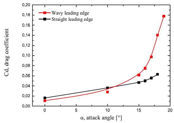
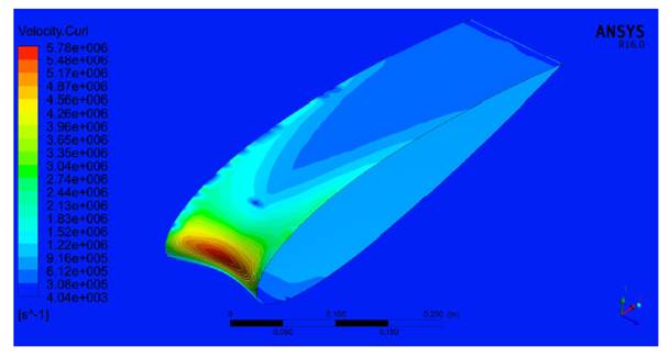
Regarding the drag force change with angle of attack obtained by the numerical simulations as shown in Figure 7. For small angles in the range 0^◦ < α < 12.5^◦, it can be noted that the drag coefficient of the WLE airfoil is in the same order if compared with the corresponding drag of the SLE airfoil. However, as the angle of attack increases approaching the stall condition, approximately at α = 15^◦, the WLE airfoil presents a drag coefficient 31.1% greater than the corresponding SLE airfoil. This increase of the drag coefficient in the airfoil with WLE for high angles of attack may be explained by the presence of flow re-circulation in the trough of the wavy leading edge, which is clearly seen from the vorticity field shown in Figure 8.

Figure 7 Comparison Cd vs. α for SLE and WLE configurations 

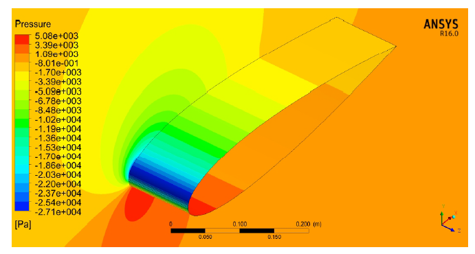
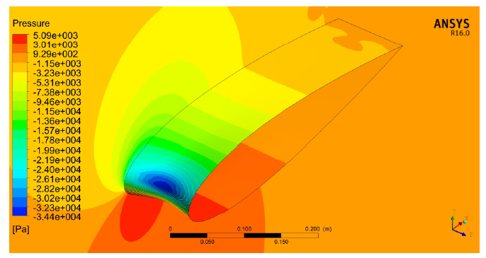
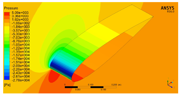
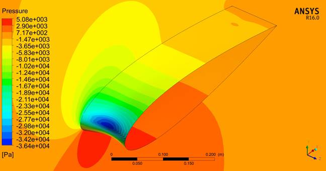
Figures 9 to 12 exhibit the pressure fields in the pre-stall regime (angles of attack of 17 and 18 ^◦ ), for SLE and WLE, respectively (in fact, considering the pre-stall regime of the WLE configuration).

Figure 8 Vorticity magnitude field for WLE, α = 15 ^◦  

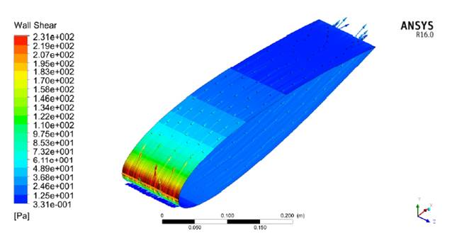
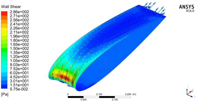
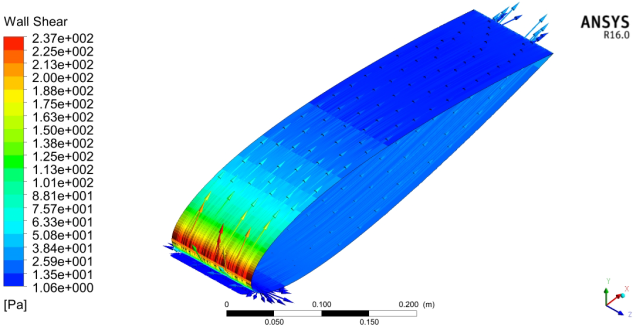
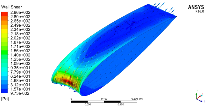
It is observed that the change of geometry for the WLE produces an adverse pressure gradient in a direction not parallel to the flow generating vortex parallel in the surface of the airfoil. This adverse pressure gradient increases the intensity of the shear stress being responsible for the reduction and stabilization of the recirculating flow region (seen on the wall shear stress fields of Figures 13 to 16), and, thus, the lift enhancement. As a consequence, the low inertia of the fluid boundary layer, which is transported away by a secondary flow, is replaced by a higher momentum fluid of the recirculating flow. This re-energizes the boundary layer behind each chord peak, as such, delaying flow separation.

Figure 9 Static pressure field for SLE, α = 17 ^◦  

Figure 10 Static pressure field for WLE, α = 17 ^◦  

By comparing the pressure coefficient distribution along

Figure 11 Static pressure field for SLE, α = 18 ^◦  

Figure 12 Static pressure field for WLE, α = 18◦ 

Figure 13 Wall shear and vector velocity plot for SLE configuration, α = 17 ^◦  

Figure 14 Wall shear and vector velocity plot for WLE configuration, α = 17 ^◦  

the airfoil surfaces for both configurations for an angle of attack 18◦, as depicted in Figure 17, it can be noted that

Figure 15 Wall shear and vector velocity plot for SLE configuration, α = 18 ^◦  

Figure 16 Wall shear and vector velocity plot for WLE configuration, α = 18 ^◦  

the initial part of the wavy profile has a higher value of negative pressure, which generates an enhancement of lift force. However, the higher negative peak values produce a stronger adverse pressure gradient, inducing the flow to be more prone to separation. In spite of it, the flow keeps attached at leading edge due to the recirculating flow from the WLE, which injects higher momentum from the upstream re-circulation. As a consequence, the stall condition is delayed for the WLE configuration by 3 degrees, i.e., an increase from 15 ^◦ to 18 ^◦ of the stall angle, as well as of the maximum lift value.

6. Conclusions

In the present work, the effects of a tubercled leading edge in a high Reynolds regime were investigated by means of numerical simulations based on the RANS equations solution (Spalart-Allmaras turbulence model). The tubercled configuration is based on the NACA 0021 airfoil profile with a wavy leading edge (WLE) of 11% wavelength and 3% amplitude both with respect to the airfoil chord. From the numerical results, it can be concluded that the presence of WLE, at least for the configuration considered, contributes to increase the maximum lift coefficient, also reaching a higher stall angle in comparison with the baseline NACA 0021 profile with straight leading edge (SLE). However, a considerable increase in the drag coefficient for the WLE configuration has also been observed. Such behaviour may be explained by the recirculating flow formed at valleys of the wavy leading edge, which injects momentum into the adjacent boundary layer, and, thus, delaying flow separation.

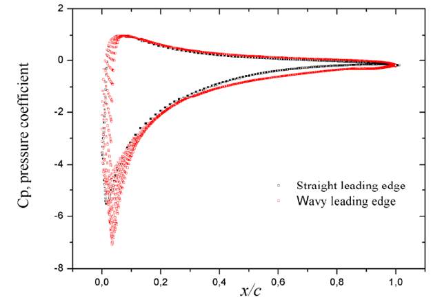
Figure 17 Cp, pressure coefficient, on the airfoil surface along the chordwise direction, x, of the configurations with SLE (Straight Leading Edge) and WLE (wavy Leading Edge) for angle of attack α=18 ^◦  

In this context, the installation of such flow control technique with wave leading edge airfoils has a potential contribution to increase the maximum lift as well as the stall angle, however, at the expense of an increase in drag.

Finally, it should be noted that the flow has been obtained numerically by RANS based equations, hich does not take into account the smaller scales of turbulence, as such, limiting the precision of the solution, especially at high angles of attack, beyond the linear lift slope curve. Therefore, the use of DES (Detached Eddy Simulation) and LES (Large eddy simulation) equations, which considers the effect of smaller turbulence scales as well as withstand highly unsteady flows, should be considered for future investigations, as such, providing more detailed and accurate solutions, in particular, when the flow condition is the pre-stall and post-stall regimes.