


 English (pdf)
 Article in xml format
 Article references
 Send this article by e-mail
 Cited by SciELO
  Cited by Google
  Similars in
SciELO
Similars in
SciELO  Similars in Google
 Permalink
1. Introduction
In recent years, humanity demands a large amount of electricity; Latin America, for example, has a growth rate of 5% [1, 2] The use of raw materials, the cornerstone of technical progress in the middle of the twentieth century, to satisfy consumption contributes to the erosion of nature and to promote anthropogenic climate change. In this scenario, renewable energies are incorporated as a new actor trying to cover what society requests in a less polluting way.
There are essentially two schemes where renewable production is present. The first, distributed energy resources (DER), includes different aspects such as generation, storage, and demand response; an interesting case study of the latter aspect is discussed in [3]. On the other hand, the new paradigms and the latest developments in the electricity sector are based on the introduction of distributed generation (DG), which is a philosophy where energy is not produced exclusively in large centralized plants, if not also in smaller locations taking advantage of local conditions in order to minimize transmission/distribution losses, as well as optimizing production and consumption. This represents an opportunity for renewable energies, where elements such as photovoltaic panels and wind turbines, scattered throughout the network, supply installations on-site or sell energy depending on their generation/consumption conditions [4]. Consequently, according to data from the European Commission, DG penetration into the European network is estimated to be around 20-25% of the total generation by 2020, and by 2030 this figure will be set at 30-35%.
However, electricity generation based on renewable resources, mainly wind and solar, has highlighted additional challenges in the management of the electricity system, primarily due to the dispersion of this type of generators, the energy of changing output, and the inefficient coordination of the conditions of the electrical grid. These complications have created technical obstacles such as energy management, architecture design of electrical systems, voltage, and frequency support, means of protection and low voltage aspects [5]. They also increase the computation difficulty due to the more complex and asymmetrical probability distributions associated with the intermittent plant [6]. In addition, given the considerable number of plants, there is the challenge of obtaining energy production data in real-time [7]. Other relevant issues are the difference, in statistical terms, between the availability of intermittent source resources and conventional generation, as well as the contribution that oscillating production can make to satisfy the peak demand of the system while maintaining its reliability [8].
Complications caused by photovoltaic generation are dependent on solar radiation, promoting the interest of different studies to find a probability model that best fits the measurements. Thus, [9] performs a radiation analysis in Taiwan with Weibull distributions, logistics, Normal, and logNormal without detecting bimodal behavior. Additionally, in [10], they claim that the variation in radiation does not follow bimodal behavior. In addition, the study of the behavior of global radiation in the M’Sila region (Algeria) is developed in [11], using six individual frequency distributions finding that the Weibull distribution best matches the measured data for all months, that is, they did not find a bimodal fit either. On the other hand [12, 13] argue bimodal performance in the distribution of radiation observations, [14] they analyze solar radiation records and similarly detect bimodal behavior in the distribution of data for intervals less than 60 minutes.
Given the importance of photovoltaic generation, this work attempts to approximate the quantification of the real power supplied from photovoltaic arrays (PVA) to the microgrid of the Center for the Development of Renewable Energies (CEDER) belonging to the Center for Environmental and Technological Energy Research (CIEMAT) located in Soria, Spain. The analysis focuses on modeling, on a monthly basis, the radiation with the Gamma probability distribution and, at the same time, finding relationships between it and the individual production in days with the best solar resource finding the profile of each PVA.
The text is made up of four sections. It begins with the description of the components of the case study and the elements for measuring the information. Section three shows the methodology for modeling radiation and determining the association functions between the solar resource and the PV power. Point four exposes the results of the characterization of the monthly radiation and the representative functions of the behavior of the PVA validated by the JMP version 8.0.2 software as well as by the measurement approach index (Ipm), in addition, the simulation of the monthly power of the PVAs is presented with the help of Matlab R2015a, it is important to note that some of the results presented in this article are published in [15], Finally, the most relevant conclusions are presented.
2. Case study
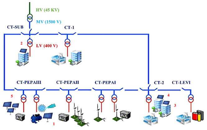
Of all the manageable components of CEDER’s microgrid, this work focuses on a photovoltaic generation whose total peak power is of 78 kW. As shown in Figure 1, the PVAs are assembled into five generation groups [16], three of them are on roofs and the rest are at floor level.
The five solar sets are briefly described.
Turbine zone: the installation consists of 16 kW distributed in 64 panels of monocrystalline silicon of 250 W each, housed in two structures, forming four series (two series per structure) of 16 panels each. The output is connected to a 15 kW inverter and connected to the three-phase network.
Roof photovoltaic building E01 Arfrisol: this generator of 12 kW is made up of 80 monocrystalline silicon panels of 150 W, distributed in five series of 16 modules each. They arrive at a three-phase inverter of 10 kW.
Building roof E03: the arrangement has a power of 12.5 kW in 54 panels of monocrystalline silicon of two different brands. Some give 230 W and the other 240 W, with very similar characteristics, there are 36 of the first type and 18 of the second. They are connected to a 10 kW three-phase inverter.
Building roof E09: plant divided into two groups, one of 84 and the other of 154 modules, arranged in 17 series of 14 panels each, with a peak capacity of 23.5 kW. The 238 panels are thin film (CdTe) with a power of 97 W and discharge to a three-phase inverter of 20 kW.
PEPA III: consists of three facilities called park 1, park 2, and park 3. They deliver their generation to single-phase inverters of 5 kW, connecting each park to a phase. Structures 2 and 3 are the same. Park 1: consists of 24 modules of polycrystalline silicon distributed in four series of 6 panels, its peak power is 5 kW. Parks 2 and 3: generators of 32 modules of monocrystalline silicon of 140 W, grouped in four series of 8 panels, providing a maximum power of 4.5 kW.
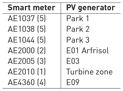
Due to the need for higher resolution data, the measurement of the solar resource in situ was performed with a station belonging to the Response Surface Radiation Network (BSRN) whose purpose is to detect relevant changes of this variable on Earth that are related to climatic changes [17]. The equipment is located in building E01 and measures various parameters such as UVA, UVB, infrared, etc.; however, only global radiation is of interest for this work. The information was acquired every five minutes in the period from November 1st, 2010 to May 15th, 2015, with a total of 442,905 records. The monitoring of the power injection produced by the photovoltaic plants to the CEDER network was done through intelligent meters; their acquisition is exported to a database formed at different granularity, 5 minutes, and hourly, respectively. The correspondence between the measuring equipment and its respective PVA is presented in Table 1.
3. Materials and methods
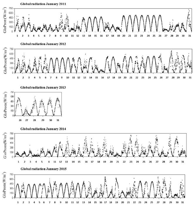
Before visualizing the developed methodology, Figure 2, as an example, presents the evolution, without processing, of the radiation in January. As can be seen, the complete history of the measurement records was not available. In addition, it is easy to observe the oscillation in the values of the solar resource for different days of the month.
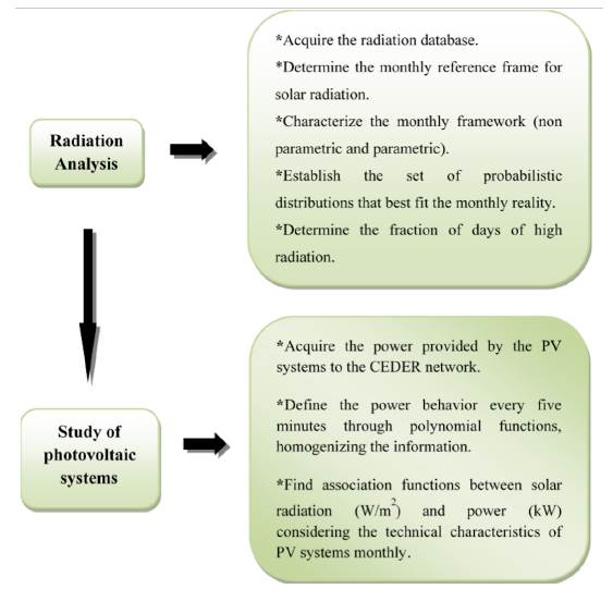
In order to facilitate the understanding of the methodology developed and the variables involved in it, Figure 3 shows the corresponding flow chart. Lines below deepen these sections.
3.1 Radiation modeling
Gamma distribution
Since the behavior of a random variable is described by its probability distribution, the closest to the measured monthly radiation was sought. Among the most useful for representing atmospheric parameters is Gamma, which is suitable for modeling when bias, positive asymmetry, and time is involved. Such environmental measures include precipitation, wind speed, and relative humidity, all restricted by a physical limit.
In short, the Gamma distribution is the one where the random variable occurs α times until there is a certain event [18]. Its density function is given by Equation 1:
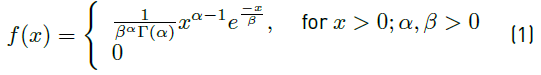
Where α is the shape parameter and β the scale parameter. When large values of α occur, distributions result in less bias and a shift in the probability of density to the right. For very large values of α (50 < α <100) the distribution approximates, in its form, the normal. The parameter β “extends” or “squeezes” the function to the right or to the left, when β is large, the curve is more elongated [19] .The main cases of this distribution are as follows: with α < 1, it is strongly skewed to the right. For α = 1, the function cuts the vertical axis in 1/β with x = 0 (in this scenario is called exponential distribution). With α >1, the distribution begins at the source, (f (0)= 0).
To model the radiation, the analysis was carried out with the Normal and Gamma distribution, individually and in combination, that is, two Normal distributions and two Gamma, respectively. The JMP software was used, filtering the information for each month, with a granularity of 5 minutes and limiting the records to the existence of radiation. In the first two analyzes, the Kolmogorov - Smirnov - Lilliefors (KSL) and Cramer-Von Mises (CVM) goodness of fit tests are applied to determine whether or not the null hypothesis is rejected. In the case of gamma behaviors, the curve adjustment goodness test was developed using Pearson’s statistic by simultaneously quantifying four parameters, obtaining the observed frequency directly from the measurements and testing the parameter values by adjusting them to create a minimization of the χ2 statistical. The process of obtaining the parameters, for each month, was carried out in the Excel program so that this test maximized the probability of the right tail of the same χ2. The hypothesis test applied in the adjustment goodness adequacy is:
Create classes in the histogram. There are as many classes as 5-minute measurements exist in each month.
Locate the original data in each class, i.e., the observed frequency (fro) is found.
Create the hypothesis test (HT). H0: Do the original data follow two Gamma distributions with their parameters αa, βa, and αb, βb? H1: does not comply with the above.
Prepare the expected frequency table (fre).
Calculate the statistical
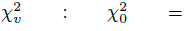 . Where: ν represents the degrees of freedom (DF). ν = k - P -1, with k the number of classes and P the parameters to be determined.
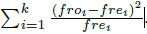
The criterion for rejection of H0 is: χ2 0 ˃ χ2 v,a .
If it is not possible to reject, we can assume, with the confidence of (1-α) % that the data set does meet the double Gamma distribution.
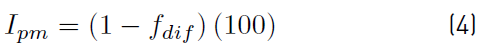
Approach index to measurements
In order to demonstrate the reliability of radiation simulation, an indicator was established to demonstrate proximity to measured data. The proximity index to measurements (I pm ) is defined with the help of the Equations 2 - 4:
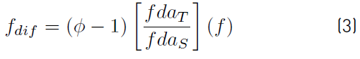
Where ϕ is the ratio of the simulated reference splines (dr
pS
) and the theoretical one obtained with the information (dr
pT
) [20], ( f
dif
) is the fraction of difference and is a function of the fractions of days of good theoretical radiation (fda
T
), of that provided by the simulation (fda
S
), and of the random
 where σ
2 is th e variance of the combined simulation of the crossed gamma adjusted to the nearest integer.
where σ
2 is th e variance of the combined simulation of the crossed gamma adjusted to the nearest integer.
A fraction of high radiation days
To determine the percentage of days with better radiation were found two monthly values, these are: reference distance (rd) represented by the radiation peak measured from the spline reference frame and high distance (hd) estimated from the points observed with the highest magnitude. In this way, the fraction of high radiation days was found:
 . When there are days of higher radiation, the spline "rises", thus both distances are close, indicating the presence of a greater number of days where the radiation is considered high.
Radiation conformation
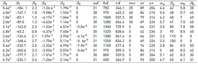
The structure of the monthly radiation matrix (Rad), which represents the 12 months of the year, consists of 192 elements consisting of 12 rows and 16 columns. Its configuration is as follows: the elements located in the first six positions correspond to the β’s of the polynomials of each month, obtained from the characterization of radiation [20]; the number of days (nd) is found in column seven, the following three parameters are the maximum reached value, that is, the peak radiation (pr), the magnitude of the reference spline (rd) and the minimum value (mv). The start (sr) and end (er) readings of the radiation measurement form columns eleven and twelve and the last four are the coefficients of α and β of the two Gammas distributions; in this way, αa and βa equal the simulation on sunny days and αb and βb represent the cloudy days.
3.2 Photovoltaic systems
Standardization of PV power
The analysis of the solar systems was carried out in two parts, the first, directly relating the radiation, on the days with the best resource (the PV systems in their design are independent of environmental variations in their operation), and the production of the measured AFVs by the following equipment: AE1037, AE1038, AE1044, AE2000, and AE2005. It is important to remember that the systems measured by AE1038 and AE1044 correspond to exactly the same facilities in their architecture and type of technology. However, energy variations were found in four months, and consequently, the analysis of the park two only covers the months of July, August, September, and October. The second section corresponded to the characterization of the power obtained by the meters AE2010 and AE4360; different polynomial adjustments without transformation were tested finding few correlations, so it was decided to analyze the transformation with logarithm base 2 in the response (power) to improve the experimental space of measurements to represent its behavior clearly. The reason for using transformation with base logarithm 2 instead of the traditional natural logarithm was to observe improvement in correlation by reducing the base exponent e to 2, better adjusting both curves to the “m” type characteristic. The statistical criterion of choosing base 2 is supported on the Box-Cox Y Transformation technique that minimizes the sum of squares of the error in the response [21]. Equation 5 shows the arrangement of Box and Cox.
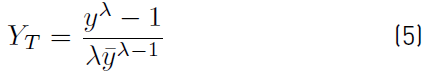
Where y is the geometric mean and λ is an exponent that varies between -2 to 2.
In this way it is possible to determine the behavior between the generated energy and the measured radiation, homogenizing the information every five minutes.
Association Functions (r’s)
The monthly relationship between the measurements of energy produced and radiation received is found with polynomial functions in the form of reasons that allow it to be segmented to any granularity. Since each PV system has its nominal power referenced at 1,000 W/m2, the peak functions (rp) are obtained. Thus, we have Equations 6 and 7:
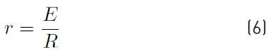
Where r and r
p
are the associations between the energy produced and the radiation at a certain instant and in peak conditions, E is the energy measured by the smart meters in Table 1, R represents the measured radiation, E
p
and R
p
describe the energy and radiation in maximum conditions. It is worth mentioning that in the PVAs of higher production, the functions r and r
p
were converted again with the help of the following property of the logarithms:
 .Where a is the basis of logarithm and N is the number to be transformed. Of this mode r is a function obtained from the best moments of energy measured with their respective radiation, that is, in each month and in each PVA the best production was sought because at that time it is when there is a greater approach with the exposed by the manufacturers. For its part, r
p
is a constant associated with the maximum values of energy delivered to the network with the moment of the best radiation. From the above, it is possible to determine the simulated power (kW) of each of the PVA by means of Equation 8.
.Where a is the basis of logarithm and N is the number to be transformed. Of this mode r is a function obtained from the best moments of energy measured with their respective radiation, that is, in each month and in each PVA the best production was sought because at that time it is when there is a greater approach with the exposed by the manufacturers. For its part, r
p
is a constant associated with the maximum values of energy delivered to the network with the moment of the best radiation. From the above, it is possible to determine the simulated power (kW) of each of the PVA by means of Equation 8.
Where P sim is the simulated power (kW), P n is the rated power (kW) of each FV system, Rad sim is the radiation (W/m2) that the simulator generates. However, where radiation exceeds 1 kW/m2 the PV production shall be higher than the nominal one.
4. Results
4.1 Radiation
Normal and Gamma distributions
First of all, the adjustment with the normal distribution was developed, the KSL test was applied and the H0 was rejected, later, the Gamma distribution was tested, and this, without a doubt, is better approached to reality; however, the CVM goodness test also rejected H0. For simplicity, it has been decided to show only the radiation behavior of January through a histogram with their respective classes. Figure 4 shows the adjustment of the Normal distribution and Figure 5 the corresponding analysis with the Gamma distribution, each with their respective tests of goodness of fit.
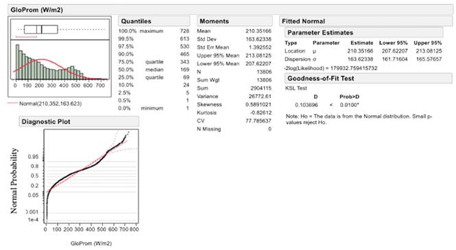
The reason for rejecting the adjustment of the normal distribution lies in the following fact: under this behavior, the average and the standard deviation of the data represent the possible best fit; clearly in the figure, the null approach is observed.
When an asymmetric distribution, such as Gamma, is applied to the information, the methodology for achieving the best possible adjustment consists in optimizing the shape parameter (α) since it represents the region of greatest probability (area under the curve) and obtaining the average of the data to estimate the value of the scale parameter (σ), due to the above, in the figure, there is a better visual adjustment in the upper part and in the asymptotic low zone there is a mismatch. However, the proximity is greater compared to the normal distribution.
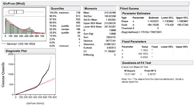
On the other hand, statistically, the likelihood parameter [-2log (Likelihood)] estimates how good the adjustment to the observed points is; the smaller this value, the better the proximity ; under this criterion the Gamma distribution represents greater proximity to the radiation behavior. In addition, in the quantile diagram of Figure 5 approximately up to 450 W/m2 there is a good coupling, above that value the distribution no longer behaves properly. That is, globally the Gamma setting is better. By reviewing the behaviors of the experimental points and histograms, it was detected that there is no single distribution; that is, there are two different probabilistic behaviors. Visually the first behavior, between 0 and 350 W/m2, tends to be a gamma with α = 1 (exponential), and the second to a normal one, its combined effect would generate the histogram of the data.
The above combination was tested without the expected response. Due to this, two normal curves were associated, being equally rejected. When this possibility was ruled out, two crossed Gamma distributions were tested: the first represents the days of low radiation and the crossed represents the one with the highest solar resource. When carrying out different tests, combining them, and varying their characteristic parameters, the strong approximation is observed with the radiation measured in each month, generating them without spaces that serve as input for photovoltaic systems.
Radiation simulation with Gamma distributions
To find the parameters of the Gamma distributions that produced a closer approximation to the radiation, four simulations were performed, creating four years of radiation. Figure 6a shows the behavior of the observed points and the spline fit with their R2. Where “X” is the reading number (NL) and "Glo" is the radiation for the month of January. In contrast, Figure 6b shows 15,000 simulated points every five minutes of radiation, as well as its spline approach that reaches a correlation factor
 of 0.7141, exceeding what was found in the observed data. The main difference in the correlation factor is the number of points, that is, in the acquisition of information there are absences of records. A criterion taken into account to get closer to reality was to keep the spline function at the same original value, that is, for this month the peak of the original data is 350 W/m2 and 346.157 W/m2 was reached in the simulation. In other words, there is a difference of 1.11%.
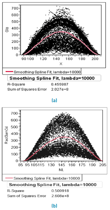
Figure 6 (a) Radiation measured in the month of January. (b) Radiation simulation with two Gamma distributions with their corresponding spline fit for the month of January
As seen in Figure 6, the Gamma density function allows the generation of random values and, consequently, the approach to the real values of the radiation. In all the months, except July and August, a double modeling is carried out because there are, notably, days of high radiation, reflected by the cross Gamma, and days of low solar resource, shown with the positive asymmetry curve. The parameter values for each Gamma are found in the Rad matrix. Figure 7 shows the two Gamma probability density functions applied to the month of January. It is observed that the crossing of both functions is very close to the value given by the spline (350 W/m2).
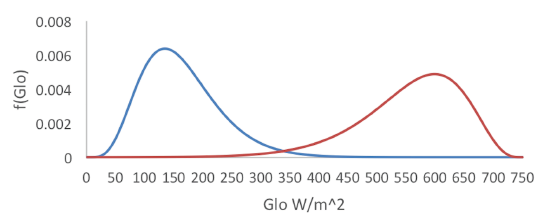
The reason for not using the Weibull distribution, although it is very flexible in its form, is the drawback of re-parameterizing the horizontal axis, being equally necessary the crossing of two functions, but with different "scales" in it.
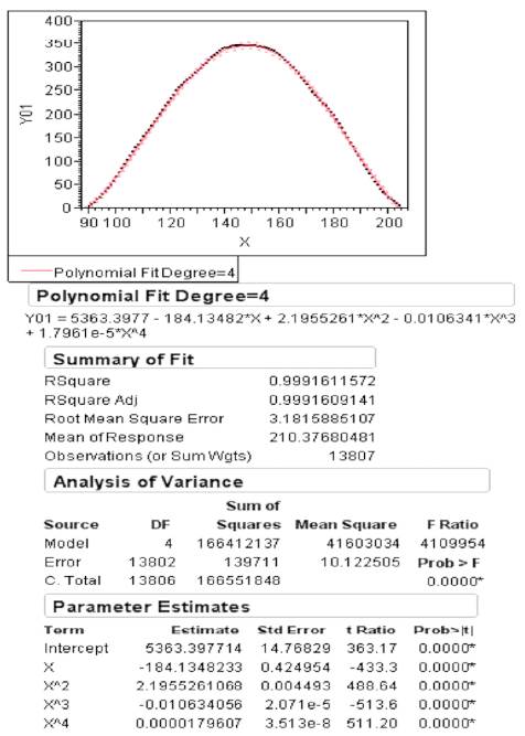
For the characterization of the spline reference frame, polynomial approaches were used. Figure 8 shows the one achieved for the month of January, where "X" is NL and "Y01" is radiation. The correlation coefficients for the remaining months are found in [22]. It is easily observed that the 4th order polynomial achieves a very high adjustment with a R2 determination value of 0.999. This function is used in the Rad matrix.
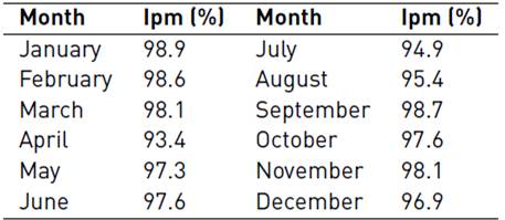
In another order of ideas, they were simulated 10 times each month to determine the Ipm; Table 2 shows the values of this indicator. As shown in the table, no Ipm exceeds the measured by 10%. April is the month where the difference is greater with 6.6%, due to intermittences of great duration, and in the months with low temperatures, the simulator is closer to the measurements.
Matrix Rad
The matrix that was formed for the simulation of the particular radiation of each month is presented in Table 3. The simulator automatically decides the section of the matrix from which it will take the information when requesting the generation of a certain month. As a characteristic of the polynomials, a majority of negative odd coefficients are observed in contrast to the pairs; this means that, odd-order contributions compensate for the increasing increases off even contributions. Since all functions are of 4th and 5th order, at least 3 curvature changes are possible, reflecting the radiation behavior. The parameters α and β of the Gamma distributions are highlighted in the matrix.
4.2 Photovoltaic generation
r’s function
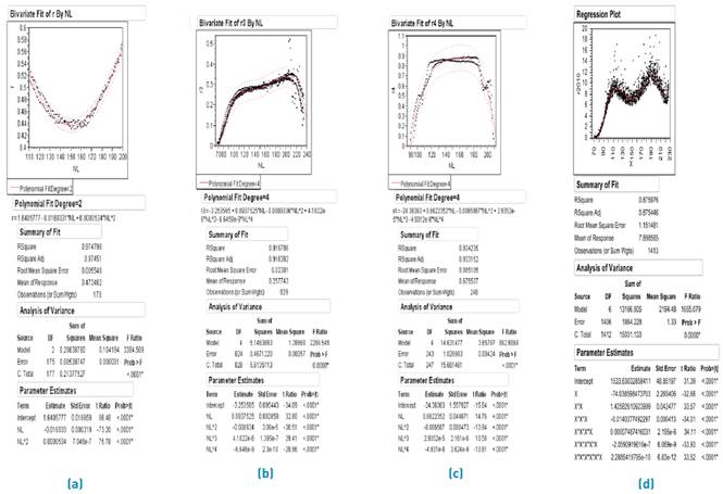
With the intention of exposing the three typical behaviors, it has been decided to present models of the functions found with their statistical analyses. For this, Figure 9 shows the functions for four PVAs measured by AE1037 (March), AE1044 (June), AE2000 (February), and AE2010 (April), respectively.
The characterization of the functions r’s of the first PVA shows, on the one hand, the best adjustments in the months of March and December, with coefficients R2 of 0.97 and 0.92 respectively; on the other hand, the approaches with less quality in the prediction are the months of May, July, and September. Relations in parks 2 and 3 show better correlations between 0.91 and 0.99. In the three PVAs of lower power perfectly marked behaviors of “U” prevail in the “cold” and “M” in the “hot” months. The best correlations, in general, coincide in the fourth PVA and at the same time, their characterizations are more complex (4° and 5°), in the months where the temperature is low they have perceived behaviors in the form of “Ո” and under this trend, the results are better, averaging R2 determination coefficients of 0.935. In Figure 9d, although the shape does resemble the “m” shape, two maxima are clearly differentiated, which represent greater effectiveness in the conversion. It is visible that the degree of function is higher in relation to smaller PVAs. The latter system has greater diversity in the behaviors found, however, it is still the high order functions that best fit.
It is emphasized that in each of the analyzes meaningful relationships (α ≤ 0.05) are met and all the estimated parameters satisfy the tests of statistical behavior causing the regression.
Photovoltaic power simulation
Although the simulator has an interval where the user can request different powers of the PVA, it was decided to use the CEDER nominals to compare the simulation with its consumption, the period requested was one year. Table 4 shows two of the most important characteristics: Fhr is the factor of days where the radiation is greater than the reference spline and Ppmed corresponds to the average peak photovoltaic power of all PVAs.
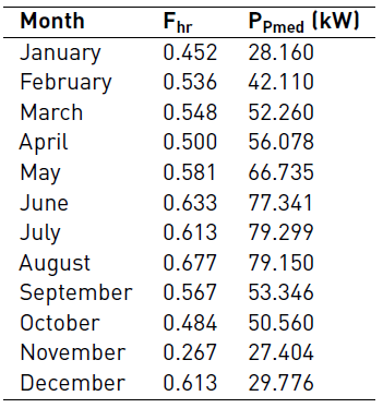
The Table 3 shows three months that would not cover, on average, the maximum power of the CEDER (40 kW). For its part, the summer months would supply this requirement without any difficult, it would even be necessary to define which solar generators would interrupt its connection to the microgrid. The above is clearly, reflected in the Fhr, with an exceptional case being December, reaching 8.3% of days above the expected. During the months of June-August, Ppmed reached the nominal PV power installed. As the simulation reflects, lower production is frequently present in November.
5. Conclusions
The simulation with the crossing of two Gamma probability functions, using little processing time, reflects the best approximation of the monthly behavior of the measured radiation. This certainty allows us to affirm that the found powers PVA are reliable and, at the same time, with the relationships obtained, are include factors such as the type of solar technology, geometry of the solar assemblies, wiring losses, dirt degradation, and aging. All of the above has allowed us to establish, approximately, the capacity of the backup system necessary in each month to satisfy the electrical demand of the CEDER, at the same time, the results obtained will be raw material in the development of energy management for the same microgrid.

