


 Inglês (pdf)
 Artigo em XML
 Referências do artigo
 Enviar este artigo por email
 Citado por SciELO
  Citado por Google
  Similares em
SciELO
Similares em
SciELO  Similares em Google
 Permalink
1. Introduction
The effect of inventory costs on the strategic design of supply chains has not been fully studied. Network optimization models frequently exclude inventory decisions and costs[1]. Several works that deal with network design do not consider inventory holding costs for decision making[2, 3].
The supply chain inventory problem is twofold. First, supply chain optimization models are often deterministic while demand forecasting methods and inventory control models are stochastic. Second, optimization models for supply chain design are mostly linear or mixed-integer linear whereas demand forecasting and inventory control models are almost always non-linear.
It is common to find multi-period supply chain optimization models that consider inventory decision variables in balance constraints with or without specified inventory policies, such as prior setting of safety inventory. For example, an inventory policy may be to hold, at the end of each time period, a specified percentage of the expected demand of the next time period. Examples of these modeling strategies can be found even in recent works such as[4].
Determining how inventory levels fluctuate when a supply chain expands or contracts is not straightforward. As stated in[5], the problem is that the impact of the consolidation or expansion of supply chain inventory locations on overall supply chain inventory depends on the specific inventory control rules applied at each location. Since these rules are normally applied on an item-by-item basis and a company may be holding hundreds or thousands of items at each location, in practical applications, the problem might be cumbersome. Therefore, one way to deal with this difficulty is to find expressions, known as ‘turnover curves’, that relate average total inventory with warehouse throughput in a practical way[5-8]. Some of these curves propose linear and potential relationships that will be further applied here. In addition, extensive simulation experiments to determine turnover curves for different inventory control systems are presented in[8]. However, no supply chain optimization model was formulated in these articles.
Several authors have taken into account inventory costs in supply chain design. In a typical example, the authors formulate a non-linear-mixed-integer model to design a distribution network with a plant or central warehouse, regional warehouses, and retailers or demand zones. A single product and an (s, Q) inventory control system are considered, yielding a non-linear objective function. The model is solved using a Lagrangian relaxation procedure and the sub-gradient method[9].
A mixed-integer supply chain optimization model that considers inventory costs using the Square Root Law (SRL) is formulated in another work[10]. In general, the SRL establishes that the inventory at N locations is equal to the inventory at one location multiplied by the square root of N. According to the authors, as a result of the level of aggregation used in network design, the assumptions behind the SRL are justified in this case. The authors conclude that, when considering inventory costs in supply chain design, the optimal number of warehouses is reduced in comparison with approaches that do not consider such costs. Another contribution of this research is that network configuration for C items might be different from that for A and B items because the demands of the former are normally more erratic. This suggests that, when analyzing the effect of inventory costs in supply chain design, it is important to consider items with different coefficients of variation of demand as is the case in practice.
Other papers such as[1] present applications of inventory control and simulation models connected to supply chain optimization models to configure a large sporting goods supply chain. The authors apply a nonlinear relationship between inventory holding costs and warehouse throughput, similar to the one provided by[5]. However, the authors linearize this relationship with a piecewise linear function using binary variables. In the present article, on the contrary, the relationship is kept as nonlinear and global optimization solvers are applied to solve the resulting nonlinear optimization models. In addition, the authors apply systems dynamics to simulate forecasting and inventory control systems. In this work, a Monte Carlo discrete simulation model is applied to mimic the inventory control system used at warehouses.
Although the Economic Order Quantity (EOQ) underlying assumptions are very difficult to satisfy in practice, some works such as[11] apply it for the supply chain expansion/contraction analysis. Indeed, the authors conclude that most companies do not satisfy the assumptions for the SRL to be applicable and refer the reader to the turnover curves[5, 6, 8].
The centralization effect is commonly described by the SRL in the literature[12]. In this work, the author considers the case where warehouses are replenished by full truck loads (FTL) or by less than full truck loads (LTL) and when a fill rate to fulfill is specified. In these cases, the author claims that the SRL should not be used because the EOQ and its assumptions do not apply. (s, Q) and (R, s, S) policies are analyzed and the author considers the cycle stock and the safety stock together, that is, the total stock. The author found that the total stock varies approximately linearly with the number of warehouses for both inventory policies and for the FTL and LTL modes of transportation.
The contribution of this article is oriented towards applied research. In supply chain design, as stated before, there is not an accepted and direct strategy to consider inventory costs explicitly in optimization models. Therefore, a simulation / optimization scheme to deal with this problem is proposed next.
2. Methodology
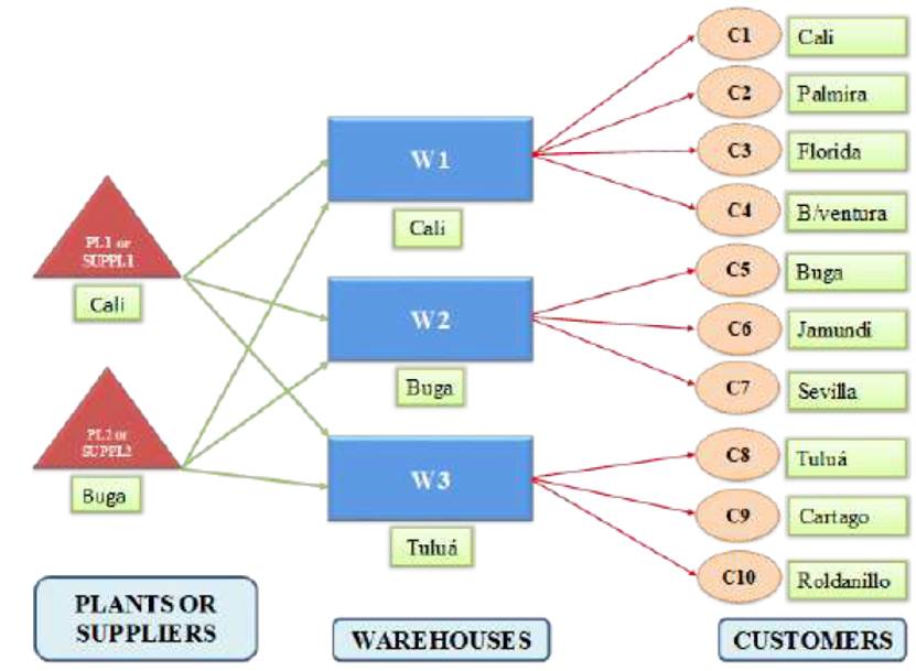
The supply chain under study is shown in Figure 1. Eight finished products are supplied from two sources that may be own plants or external suppliers. The supply chain includes three potential warehouses to be opened according to the results of the model. The warehouses ship finished products to 10 customers; each of them must be distributed from only one warehouse (single sourcing). The instances solved are carefully generated from realistic data based on a supply chain in the Valle del Cauca, Colombia.
The problem is to determine adequate ways to estimate total average inventory and the impact of inventory holding costs at warehouses on supply chain configuration. In order to do this, it was necessary to simulate the inventory control system applied at each open warehouse. Since the simulation model is a close representation of reality, the total average inventory in the supply chain is assumed to be very accurate and it can be used for comparison purposes with other more aggregated inventory estimation strategies applied in the literature.
To determine optimal or near-optimal supply chain designs, a non-linear mixed integer optimization model was also formulated. Details of the inventory simulation and the optimization models are next explained.
2.1 A Monte Carlo simulation model for the inventory control at warehouses
Since total average inventory at each warehouse and in the whole supply chain are highly related to the inventory control systems applied by a company[5], the best way to estimate inventory holding costs is to explicitly consider such inventory control systems. A Monte Carlo simulation model was thus designed to represent the inventory control systems applied in the warehouses of the supply chain considered.
The model simulates a joint, periodic inventory control system (R, S i ) applied at each warehouse. This type of inventory control system is commonly applied in the region. Customer demands for eight products are randomly generated each independently of the others; these demands are assumed to be normal for six of the products and erratic with no specified distribution for two additional products. This demand approach produces a wide variety of demand patterns with coefficients of variation ranging from around ten percent to near 180%. The erratic demand is generated in two steps, first defining whether or not a positive demand will occur from a Bernoulli distribution and then generating the value of such demand from a normal distribution. The probability of having or not positive demand may be specified in the model, yielding a desired level of intermittent demand.
Since the optimization model considers single sourcing from warehouses to customers, the simulation model can assign each customer to any warehouse to represent any optimal or near-optimal solution. This is done by means of a binary parameter that can be selected by the user, according to the solution provided by the optimization model. Once the customer allocation to warehouses has been done, the simulation model estimates average inventories (cyclic, safety and total) at each open warehouse.
The simulation model comprises four types of spreadsheets: basic data spreadsheets; spreadsheets to simulate demand of each product by customer; spreadsheets of demand consolidation at each warehouse by product; and spreadsheets that calculate consolidated total and safety inventory, total annual demand, and inventory turnover at each warehouse. The latter spreadsheets were built in units of product, in tons, and in monetary units, providing the information to compare total inventory in the supply chain according to its specific design produced by the optimization model. The simulation model comprises the following assumptions and features:
The model simulates daily demand of eight products for ten customers during a year, then consolidates each product’s daily demand at three warehouses according to the binary parameter described above, and finally yields aggregated inventory indicators at each warehouse for the whole year. The model assumes a review interval R = one week and a constant Lead Time L equal to three days.
When a customer is assigned to a specific warehouse, all the products that the customer requires are assumed to be fully handled by the warehouse. Therefore, the model consolidates the demands of each product from all the customers to be served by each warehouse by summing their individual demands. Each product’s consolidated average demand and its corresponding standard deviation are thus calculated theoretically and by means of the simulation model. First, assuming that demands are independent, average demand is the sum of the individual demand means and its variance comes from the sum of the individual variances. Second, average demand and its standard deviation are directly calculated from the consolidated demand data. The results show that these two approaches are very similar, as expected. It is important to note that demands and their corresponding standard deviation are calculated in product units, tons and currency units to be used in further calculations.
In the spreadsheets that consolidate all customers’ demands by product at each warehouse, an (R, S) inventory control system for the specific product is simulated. The basic variables and equations used for the simulation are described next.
Initial inventory
It is necessary to establish an initial inventory for each product at each warehouse to avoid artificial stockouts at the beginning of the simulation. Since the Lead Time L is set to three days, the initial inventory is calculated to satisfy demand over that period. Therefore, initial inventory is calculated as given in Equation (1). Parameters ( daily and ( 1daily are the mean and the standard deviation of product daily demand, calculated from the 365 simulated days; k is the safety factor corresponding to a specified level of service of 97.5% (probability of not having a stockout at each review cycle).

On-hand inventory and net inventory
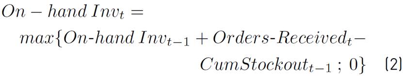
Beginning with the initial inventory, the on-hand inventory for each day t is then calculated by using Equation (2). The maximum function is necessary because the on-hand inventory cannot be negative. On the other hand, the net inventory at the end of day t can be negative and it is simply calculated as the on-hand inventory at the end of day t minus the cumulative stockouts at the end of the same day.
Stockouts and cumulative stockouts
Daily stockouts are calculated by means of Equation (3) .
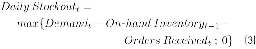
The maximum function indicates that, when the available quantity of products is greater than the demand, the stockout is equal to zero. Since it is possible that stockouts occur for two or more successive days, it is necessary to calculate cumulative stockouts so that the on-hand inventory can be correctly calculated from Equation (2) to further compute net inventory. Here, the model assumes that cumulative stockouts are never greater than the order size to receive or, equivalently, that the aggregated demand of products at warehouses is not extremely erratic. In addition, the simulation model assumes that all the stockouts are covered when a new shipment arrives, that is, stockouts are considered as backorders.
Pending orders and inventory position
Since the model considers a review interval R = 7 days and a constant Lead Time L = 3 days, each order from the supplier or plant is considered a pending order until the order arrives at the warehouse three days after it was issued. The model thus considers these pending orders to calculate the inventory position at the end of each day as On-hand inventory + On-order stock - cumulative stockouts, all at the end of the day.
Average safety inventory
The authors in[13] define safety inventory as the average net inventory just before a shipment arrives. The simulation model contains all the information to estimate safety inventory as the average of the net inventory the day before a shipment is received at the warehouse.
Average total inventory
The average total inventory at each warehouse is a key indicator to consider in supply chain design and is one of the objectives of the simulation model described above. Since the simulation model produces the evolution of daily inventory over time, the total average inventory can be estimated as the area under the inventory curve versus time divided by the total time. This area is estimated by summing the areas of the daily trapeziums and dividing by 365 days. In order to achieve the correct calculation to estimate inventory holding cost, the on-hand inventory must be considered as well as the units received when a shipment arrives.
In the spreadsheets that consolidate all customers’ demands by product at each warehouse, the theoretical values of average safety inventory and average total inventory are also included. Moreover, the order-up-to-level S is calculated based on the traditional equations for the periodic inventory control system (R, S). This S value is then used to generate the order size at each review interval as the difference between S and the corresponding inventory position.
The last spreadsheets applied in the simulation model are those that consolidate total inventories by product at each warehouse. The inventories are aggregated in units, in weight units (tons), and in currency units ($). The spreadsheet that consolidates aggregate safety and total inventories by product in tons at each warehouse is also used to estimate average total demand and average inventory turnover at the warehouse. The latter is then used to estimate average total inventory in the supply chain optimization model when considering the SRL.
2.2 A supply chain optimization model
An optimization model with single sourcing was formulated for the design of the supply chain depicted in Figure 1. The main objectives of this standard model were to analyze the impact of inventory holding costs in the design of the supply chain and to determine good approaches to explicitly consider inventory holding costs in the model. Since the model considers the products aggregated in tons, no set of products is defined. Details of the model are explained next.
Sets
P = Set of plants or suppliers (index i)
W = Set of warehouses (index j)
C = Set of customers (index k)
Parameters
PC i = Production or purchase cost from each plant or supplier ($/ton)
FC j = Fixed operating cost at each warehouse ($/year)
DE k = Average demand of each customer (ton/year)
TCW ij = Transportation cost from each plant or supplier to each warehouse ($/ton)
TCC jk = Transportation cost from each warehouse to each customer ($/ton)
N = Number of warehouses to be opened
To estimate inventory holding costs, the following parameters are also defined:
v = Average product value for items held in stock ($/ton)
r = Carrying charge for items held in stock ($/$.year)
Decision Variables
X ij = Flow of products from each plant or supplier to each warehouse (ton/year)
Z jk = Binary variable equal to 1 if warehouse j satisfies the demand of customer k; 0, otherwise.
W j = Binary variable equal to 1 if warehouse j is to be opened; 0, otherwise.
Constraints
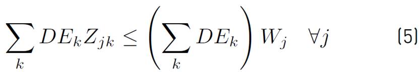
Warehouse capacity is shown in Equation (5).
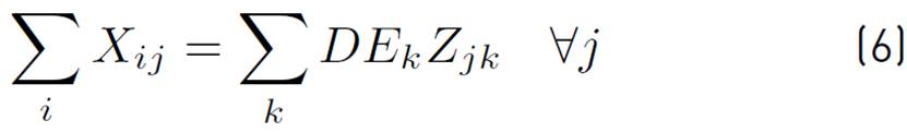
Equation (6) shows the flow balance at each warehouse.
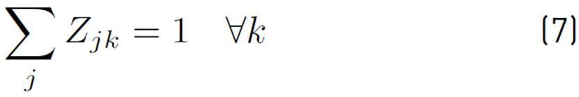
Customer allocation to just one warehouse is shown in Equation (7).
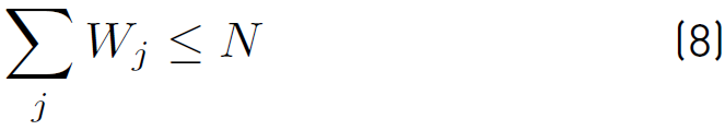
The number of warehouses to be opened is represented in Equation (8).
Variable definition appears in Equation (9).

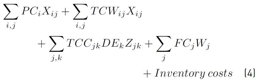
The objective function in Equation (4) minimizes total average logistics costs given by the sum of production or purchase costs, transportation costs, fixed costs at warehouses, and inventory holding costs. The latter are to be considered in different ways which will be described later. Constraints in Equation (5) allow the model to allocate warehouses to customers only for open warehouses and control the maximum capacity of each warehouse. Constraints in Equation (6) represent the product flow balance at each warehouse. Equation (7) ensures that each customer is allocated to exactly one warehouse. The constraint in Equation (8) manages the number of warehouses to be opened and, finally, constraints in Equation (9) are variable definition.
2.3 Strategies for considering inventory holding costs in the supply chain
The inventory holding costs in the objective function given in Equation (4) can be considered in a number of ways. To calculate these costs, the total average inventory held in the supply chain must be estimated. The three approaches applied here to estimate the total average inventory in the supply chain were the following:
The expressions given in[5] that relate total average inventory in a warehouse with its throughput (turnover curves).
The total average inventory in the supply chain given by the simulation model, which is supposed to be the most reliable average inventory estimation since it comes from the actual item-by-item inventory control systems applied at each warehouse.
First, the SRL uses Equation (10), where I N is the estimated average total inventory when N warehouses are operating and I 1 is the estimated average total inventory when just one warehouse is open.
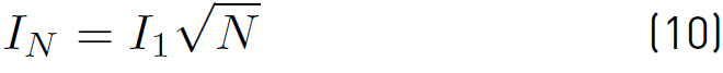
To estimate I 1, the throughput through a single warehouse is easily determined by the total supply chain expected demand and the average inventory turnover is estimated by means of the simulation model. Finally, to approximate the average inventory holding cost when N warehouses operate, Equation (11) is applied.
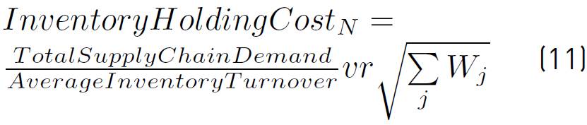
The average unitary value v of products held in inventory is also estimated by the simulation model and r is the carrying charge, which is determined by the organization. Note that the number of opened warehouses N is equal to the sum of the binary variables W j , leading to a non-linear optimization model. The authors in[10] apply the SRL to estimate inventory holding costs in a supply chain optimization model that also considers opening a number of warehouses. They reformulate the binary variables to open/close warehouses in such a way that their resulting model is a mixed-integer linear model, which can be optimally solved. Their model can also be solved by initially considering all logistics costs without including inventory costs and opening N = 1, 2, 3, …, M warehouses (where M is the maximum number of warehouses that can be opened). The inventory holding costs, calculated by the SRL, are then added to the resulting optimal objective functions, to finally find the correct optimal supply chain configuration by selecting the outcome with the least total logistics costs. Another way to solve the original non-linear model is by means of a global commercial optimizer such as BARON. When applying all the previous approaches to solve the model, the same solutions were consistently obtained. Therefore, commercial non-linear solvers were selected to solve all subsequent non-linear models, as shown below.
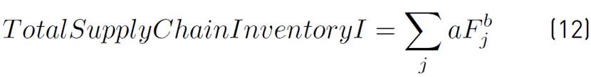
For the second approach, the potential expression proposed in[5-8] and shown in Equation (12), was applied. In this potential function, a and b are constants to be determined by least-squares regression and F j represents the warehouse j throughput. Equation (12) is valid in any warehouse of a given supply chain[5]. Therefore, this equation can be applied for different values of the total inventory I in function of the throughput F in a single warehouse and for different warehouses with different average total inventories and throughputs.
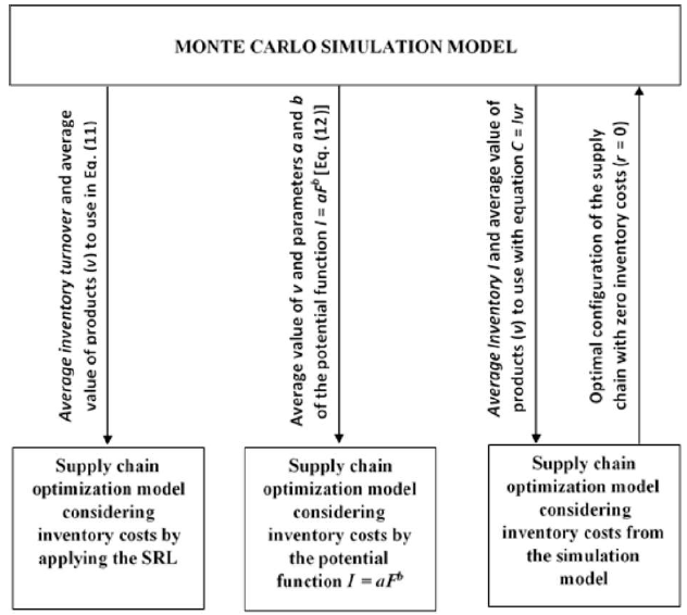
The last strategy to estimate inventory holding costs is to apply the simulation model described above. Since this model handles the real inventory control system at the product level applied at each warehouse, it gives the most reliable measure of inventory levels for any supply chain configuration. These measures are used afterwards for comparison purposes among the three approaches. The interactions of the Monte Carlo simulation model with the optimization model are summarized in Figure 2.
3. Results and discussion
The described methodology was applied in a hypothetical supply chain in the Valle del Cauca, Colombia [Figure 1], based on a careful generation of instances from real data. First, the spreadsheet of the simulation model that consolidate total inventories by product in tons at each warehouse was used to find suitable constants a and b in Equation (12).
By assigning all customers to one warehouse and varying all demands’ average and standard deviation in a systematic way, the graph in Figure 3 was obtained. A total of 30 replications were used in the simulation to estimate each pair of values for average total inventory and average throughput. Note that the coefficient of determination was R 2 = 0.9835 in contrast to R 2 = 0.9614 that was obtained by using a linear function. Consequently, the equation subsequently used in the optimization model was I = 0.024F 0.9307, where F was estimated in each case through the sum of average demands for all products and customers. In the optimization model, the throughput F j was replaced by the inbound flows to each warehouse j, using the sum of variables X ij from all sources i, and finally summing the inventory for all open warehouses in the supply chain, according to Equation (12). In this regard, it is better to use the continuous variables X ij instead of the binary variables for customer allocation Z jk because the latter complicate the solution process. It is important to observe that the above-mentioned expression considers the total inventory at each warehouse without differentiating between cycle and safety stock, a more suitable detail for practical applications.
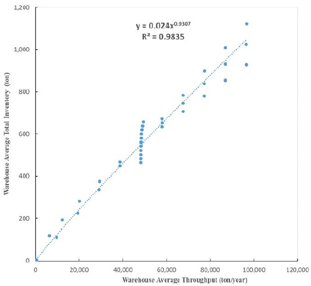
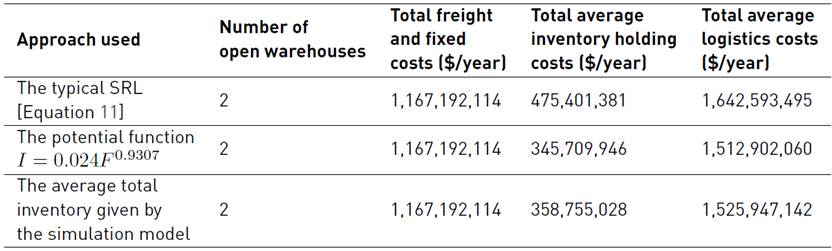
Table 1 illustrates the results of the optimization model when applying each of the three approaches to consider holding inventory costs for the configuration of the supply chain in the objective function (4). Only the average values are shown because the coefficients of variation of customer demands are very low when they are aggregated in tons. For the 10 customers considered, these coefficients of variation fluctuated from 0.94% to 1.99%. In addition, the coefficient of variation of total average inventory holding cost was as low as 0.45%, as a result of the simulation model that replicates the inventory control systems for the two open warehouses given by the optimal supply chain configuration from the optimization model. Consequently, the average values shown in the table are enough to draw some conclusions without considering statistical test of hypotheses.
Firstly, for the typical supply chain considered in this study, the average total inventory holding cost given by the simulation model is considered the most accurate of the three approaches, because it replicates the actual item-by-item inventory control systems applied in warehouses. Therefore, this inventory cost is used as a reference value. The SRL overestimated total average holding costs by 32.5% and total average logistics costs by 7.6%. In contrast, these costs only differed from the ones given by the potential function in 3.6%. Accordingly, as most authors agree, the SRL is a rough approximation of inventory holding costs in a distribution system and should not be used for supply chain strategic configuration purposes unless very specific conditions apply[11, 12].
Secondly, although the open warehouses and their allocation to customers are the same for the three cases in Table 1, all of these were run with a carrying charge r = 0.20 $/$.year. When the model was run using a variable carrying charge r from 0.00 to 0.40 $/$.year and the potential function was used, no change in the optimal supply chain configuration occurred. However, for the same range of r values, when the SRL was used in the objective function, the configuration of the supply chain changed from two opened warehouses to just one when r = 0.24 $/$.year. This result suggests that possible decision problems may arise if the SRL is applied in supply chain design.
Thirdly, when the solver KNITRO was used to solve the model with the SRL, it did not find the global solution. Instead, when using the BARON solver in the Neos Server, it reached a better solution that was 1.3% lower. There were significant differences between the two solutions because the solution given by KNITRO opened one warehouse, while the other solver opened two warehouses. A similar result was obtained when running the case for the potential function. In this case, the solver BARON reached a solution that was 0.85% lower than the one obtained by KNITRO. The difference here was only the assignment of one customer to a different warehouse because both solvers opened the same two warehouses.
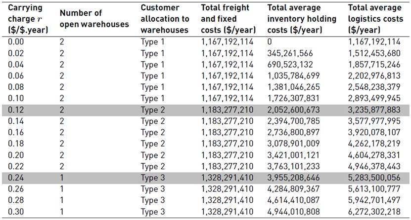
Another sensitivity analysis was done by increasing the mean product value v in $/ton and using the potential function. The original value v was relatively low and in reality, it is feasible to find much higher v values. For this reason, v was significantly increased and the model was run again varying r from 0.00 to 0.30 $/$.year. The results are shown in Table 2.
Several conclusions can be drawn from Table 2. First, estimating a suitable carrying charge r value is very important in supply chain design. Different realistic r values might produce different customer allocation to warehouses or different supply chain configurations. For this reason, a common practice that uses a rough estimate of r should be disregarded. Second, the differences in supply chain configurations can be as simple as the customer allocation to warehouses such as the change from Type 1 to Type 2 (r = 0.12), where a customer begins to be served by a different warehouse and thus transportation costs increase. Changes can also be more significant (such as the case for r = 0.24), where one warehouse is closed and the other one must supply all customers, again increasing transportation costs. All of these results suggest that including holding inventory costs in supply chain optimization by using simulation or potential curves is worth it.
4. Conclusion
A Monte Carlo simulation model to replicate warehouse item-by-item inventory control systems and an optimization model to configure a typical supply chain were formulated in this study. The main objective of these models was to analyze different strategies for including inventory holding costs in the objective function of the model. Although some results given by the simulation model can be estimated from theoretical equations, approximating those values for different supply chain configurations proved to be useful. Moreover, a simulation model can be more effective when considering stochastic lead times and perhaps other inventory control strategies that cannot be described through theoretical equations.
Since the average inventory costs approximated by the simulation model are considered as the most accurate, they were used to evaluate the performance of the SRL and of the potential functions proposed by[5-8], which relate average total inventory with warehouse throughput. The results suggest that the SRL should not be used to estimate inventory costs, unless very uncommon assumptions hold, because the SRL generally overestimates inventory costs and could yield suboptimal supply chain structures. In contrast, the potential functions that relate warehouse inventory and throughput yielded similar results to the ones given by the simulation model. Therefore, estimating and using these curves to analyze supply chain or distribution expansions or contractions is expected to be a good practice.
It is likely that, for larger instances than the ones solved in this study, some solution problems arise. Although global optimization solvers such as BARON may be helpful, further research is needed to design efficient heuristic or meta-heuristic solution procedures. In any case, considering inventory holding costs for supply chain optimization in a more detailed way should be routinely used by practitioners.

