


 English (pdf)
 Article in xml format
 Article references
 Send this article by e-mail
 Cited by SciELO
  Cited by Google
  Similars in
SciELO
Similars in
SciELO  Similars in Google
 Permalink
1. Introduction
Uncertainty is a specific characteristic of the energy sector. Although decisions in the energy sector are generally not based on predictable outcomes, some variables that affect decision making can be predicted, with certain degree of confidence, using information from different sources[1, 2].
Examples of useful information for decision making is that related to natural variables (temperature, wind speed, etc.). Information related to energy consumption and demand profiles of users is valuable too. Furthermore, new sources of renewable energy generation developed in the last 30 years are directly related to natural variables, and the corresponding information is often incorporated in prediction models for decision making[3].
Due to the aforementioned reasons, a large number of stochastic variables must be taken into account to improve operational decision making, but also to assure that the derived actions are feasible from an economic point of view. When considering a large number of variables, the complexity of the underlying models notoriously increases. However, the increase in complexity associated with the number of variables is partly compensated because the hardware infrastructure to perform computations on large volumes of data has developed strongly.
New challenges have emerged from the described reality. A very relevant one is related to the development of an intelligent system to take advantage of new sources of information and available data. Classic statistical models, that were useful for making predictions some decades ago, have limitations in this new context. Computational intelligence methods have demonstrated excellent forecasting accuracy in different areas, in recent years[4-6]. These methods are robust and tolerant to uncertainty, and they are able to learn the most relevant features of the considered data to provide a precise forecast, thus providing excellent results by excluding non-relevant information and focusing on the most useful data.
In this line of work, this article presents the application of several prediction algorithms based on computational intelligence to forecast the electricity demand of an industrial park in Spain, the electricity demand of a substation in Uruguay and the total electricity demand of Uruguay. The modeled scenarios are based on historical demand data of the industrial park (from 2014 to 2017), historical demand data of the substation in Uruguay (from 2017 to 2018) and historical total demand data of Uruguay (from 2010 to 2018). For the industrial park, a forecasting model for the next 24 hours is built by optimizing the algorithm that presented the best results for the one hour forecast.
Overall, the major contributions of the research reported in this article are: i) the evaluation and comparison of computational intelligence models applied to forecasting the demand of an industrial park in Spain, the demand of a substation in Uruguay and the total demand of Uruguay. Also ii) the optimization of the proposed models using the high performance computing infrastructure of the National Supercomputing Center, in Uruguay.
This work extends our previous article Short term load forecasting of industrial electricity using machine Learning[7], presented at II Ibero-American Congress on Smart Cities, Soria, Spain, 2019. The main contributions of the extended version are: i) a residential demand forecasting scenario applying the studied techniques on a substation and incorporating climate variables and ii) a total demand forecasting scenario of Uruguay including residential and industrial consumers. Both new instances are analyzed in order to evaluate different consumer profiles as well as different types of influence of weather variables.
The article is organized as follows. Section 2 presents the formulation of the electricity demand forecasting problema and a review of related works. Section 3 describes the proposed approach to solve the proposed problem. Section 4 reports the experimental analysis of the studied methods, and Section 5 reports analysis of the best method and extension to 24-hour demand forecast is presented. Finally, Section 6 formulates the conclusions and main lines for future work.
2. Energy demand forecasting
This section introduces the energy demand forecasting problem, describes forecasting techniques, and reviews related works.
2.1 General considerations
The energy demand forecasting problem is usually solved applying mathematical methods using historical data for prediction. There is no a general method that can be used in all types of energy demand forecasting. Thus, an appropriate method must be found for each demand profile. Using historical data of a particular demand profile is common in practice to determine the most effective algorithm. The problem can be classified by the time horizon to forecast: ultra short-term demand forecasting (up to a few minutes ahead), short-term demand forecasting (up to few days ahead), medium-term demand forecasting (up to few month ahead), and long-term demand forecasting (years ahead). Different techniques are applied when considering each time horizon. This work focuses on short-term demand forecasting using historical data.
The energy management and operation of electric grids becomes highly difficult and uncertain, particularly when new technologies are incorporated. The power demand of end customers is versatile and changes on hourly, daily, weekly, and seasonally basis. Hence, there is a real need of developing models for accurately forecasting at different time horizons, depending on the management goals.
This work focuses on both industrial and residential power consumption. Residential power profiles are usually variable, mainly depend on the time of the day and the day of the week, but they also depend on occasional vacations and other factors[8]. On the other hand, industrial power profiles tend to be stable, due to the needs of industrial processes themselves.
There are two classes of forecasting models for predicting power demand profiles: statistical and physical models. The main goal of both classes is to predict the power profile at a future time frame. Statistical models can be built for time series analysis.
They are less complex than physical models and are suitable for short term prediction. Physical models are based on differential equations for relating the dynamics of the environment and generally are applied for long term forecasting. In this article, statistical models are selected for short term forecasting due to their very good prediction accuracy and lower complexity.
2.2 Problem formulation and strategies
This section describes the problem formulation and the studied strategies for electric demand forecasting.
Relation between one hour and 24 hour forecasting.
This article focuses on applying computational intelligence methods to develop a model for forecasting electricity demand 24 hours ahead. When historical data are available with hourly frequency, is natural to develop a model that predicts next hour. From that model, a multi-step forecasting model can be constructed (i.e., 24 steps in the future).
Four strategies are typically applied for multi-step forecasting starting from a one-step model:
Direct strategies develop a different model for each time step to be predicted. Assuming past observations of the variable to be predicted are used, this strategy implies, in case of 24 steps, developing 24 models with the structure defined in Equation (1), where pred t is the prediction of time t value and obs t is the observed value at time t.
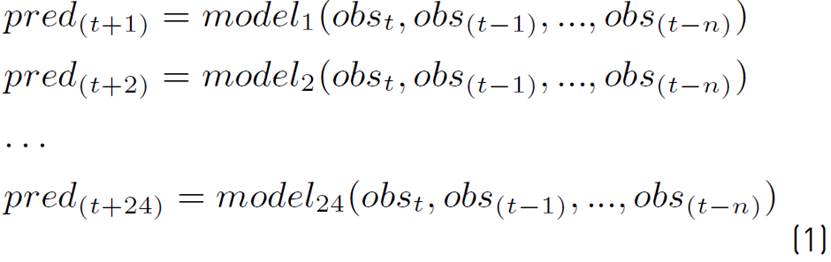
Unfortunately, a direct strategy implies developing a model for each time step to be predicted and consequently is very expensive computationally. In addition, temporary dependencies are not explicitly preserved between consecutive time steps.
Recursive strategies apply a one-step model (recursively), multiple times. Predictions for previous time steps are used as input for the prediction on the following time step. The structure to develop for a recursive strategy is presented in Equation (2).
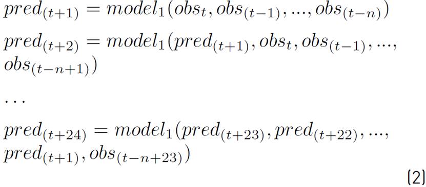
In this strategy predictions are used instead of observations. A single model is trained, but the recursive structure allows prediction of errors to accumulate; also, the performance of the model can quickly degrade as the time horizon increases.
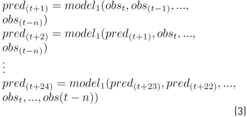
Hybrid strategies combine the previously described to get benefits form both methods. A separate model is constructed for each time step to be predicted. Each model may use the predictions made by models at prior time steps as input values. For example, using all known prediction, a hybrid strategy produces the structure in Equation (3).
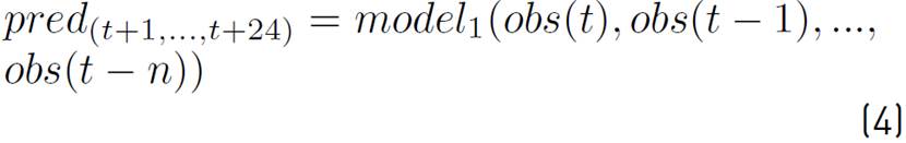
Multiple output strategies develop a model that has as output all time steps to be predicted (in this case 24). Multiple output models are more complex as they can learn the dependence structure between inputs and outputs as well as between outputs. For this reason, they are slower to train and require more data to avoid overfitting. Equation (4) shows the corresponding structure.
In this work, hybrid strategies are applied for solving the forecasting problem.
One hour forecasting model training. Section 2.3 reviews different approaches and methods for short term demand forecasting. This work explores the use of machine learning techniques, mainly those based on model ensembles. Feature selection is commonly applied in this kind of problems due to several reasons. Simpler models are easier to interpret, and have shorter training times. Also, the size of the model using less features is smaller, mitigating the curse of dimensionality[9]. But the main reason to apply feature selection is to reduce overfitting, enhancing generalization of the model to unseen data.
Once established the strategy to extend the next hour forecasting models to twenty four hours model, the main issue is to obtain the best possible model for the next hour. With this purpose, standard steps are taken: i) data gathering, ii) data preparation, iii) choosing a model, iv) training, v) evaluation, vi) parameter tuning, and vii) testing. Each of these steps is described in detail in Section 3.
Complete model. After obtaining a one-hour model with optimized parameters, it is trained for the next hour taking all steps mentioned. Thus, 24 four different instances of this model are trained, one for each of the next 24 hours. Then, the hybrid strategy described in Equation (3) is applied to build a 24-hour forecasting model. The complete model is evaluated on testing data and results are reported.
2.3 Related works
Several methods have been proposed for electricity demand forecasting, applying short, medium and long-term predictions. These methods are classified in statistical models and machine learning models. This work focuses on short-term demand forecasting using machine learning.
Most used forecasting techniques include auto regressive models (AR), moving average models (MA), auto regressive moving average models (ARMA) and auto regressive integrated moving average (ARIMA) models[10]. These kind of models are easy to implement. ARIMA models for short-term demand forecasting[11] were initially proposed by Hagan and Behr.
Taylor and McSharry compared different ARIMA implementations using load data from multiple countries[12]. Dudek proposed applying a linear regression technique[13]. However, linear models are inadequate to represent the non-linear behavior of electricity demand series and fail to predict the accurate future demand values. Thus, their forecasting accuracy tends to be poor. Some studies try to overcome the aforementioned difficulties considering nonlinear components, obtaining good accuracy metrics[14].
Several studies have been conducted on short-term demand forecasting using non-linear models. For example, Do et al. described a model for predicting hourly electricity demand considering temperature, industrial production levels, daylight hours, day of the week, and month of the year to forecast electricity consumption[15]. Results suggested that consumption is better modeled considering each hour separately. In our work, this strategy is developed and applied. Son and Kim proposed a method based on support vector regression preceded by feature selection for the short-term forecasting of electricity demand for the residential sector. For feature selection, twenty influential variables were considered and the quality of the model improved substantially[16].
Other mid-term demand forecasting studies consider variables such as GDP and prove that are highly correlated with the demand[17]. Peak demand estimation is also crucial to determine future demand, in order to assist future investment decisions[18]. In this article, the decision to consider ensemble models was taken based in the work presented by Burger and Moura, who applied a gated ensemble learning method for short-term electricity demand forecasting and showed that the combination of multiple models yielded better results than the use of a single model[19]. Silva presented a complex feature engineering to build gradient boosted decision tres and linear regression models for wind forecasting; in our work several similar ideas were developed for demand forecasting[20]. De Felice et al. applied several separate models for each hourly period. Each of those models measure variations in electricity demand based on multiple variables[21]. Recent studies in traffic prediction in the context of Internet of Things have shown promising results using advanced artificial intelligence techniques related to those applied in our work[22, 23]. Computational intelligence has also been applied to forecasting and dissagregation of residential energy consumption[8, 24].
The analysis of the related works allowed to conclude that two main issues impact on the forecasting capabilities and the results quality: the model itself and other preparation and pre-processing techniques.
Several works applied techniques like data normalization, filtering of outliers, clustering of data or decomposition by transformations[25-28] to improve prediction results.
In our research, several data preparation techniques are applied for building a robust approach for short term energy utilization forecasting. Next section describes the proposed approach.
3. The proposed approach for day ahead demand forecasting
This section describes the proposed approach to solve the day-ahead electricity demand forecasting for an industrial park in Spain, a substation in Uruguay, and for the total demand of Uruguay applying the strategies described in Section 2.2. In addition, implementation details of the proposed models are presented.
3.1 General approach
This subsection describes the data and the proposed methodology for electricity demand forecasting.
Data description, preparation, and metrics
Data description. Data for the three studied scenarios are described next. Industrial park in Burgos, Spain. The first scenario reported in this article considers historical hourly energy consumption data from an industrial park in Spain. Data were collected between January 2014 and December 2017. The dataset consists of industrial energy consumption measurements. Each measurement is composed of the following fields:
Year (integer), representing the year on which themeasure was taken.
Month (integer), indicating the month on which themeasure was taken.
Day (integer), indicating the day on which the measurewas taken.
Hour (integer), indicating the hour on which the measure was taken.
Dayofweek (integer), indicating the day on which the measure was taken.
Workingday (boolean), indicating whether the measure was taken in a working day or not.
Useful (boolean), indicating whether the measure is valid.
Demand (float), indicating the real power measured.
Substation SB1872 in Montevideo, Uruguay. The second scenario studied in this article considers historical hourly energy consumption data from a substation in Tres Cruces neighborhood in Montevideo, Uruguay. Tres Cruces is a neighborhood located near the centre of Montevideo that serves 390 citizens distributed in 117 homes with medium socio-economic level[29]. The studied dataset contains residential energy consumption measurements collected between January 2017 and December 2018. Each measurement is composed of the following fields:
Year (integer), representing the year on which the measure was taken.
Month (integer), indicating the month on which the measure was taken.
Day (integer), indicating the day on which the measure was taken.
Hour (integer), indicating the hour on which the measure was taken.
Dayofweek (integer), indicating the day on which the measure was taken.
Workingday (boolean), indicating whether the measure was taken in a working day or not.
Useful (boolean), indicating whether the measure is valid.
Temperature (float), indicating the temperature.
Humidity (float), indicating humidity.
Wind speed (float), indicating the average wind of a specific hour.
Demand (float), indicating the real power measured.
Total demand of Uruguay. The third scenario studied in this article considers the historical hourly energy total demand from Uruguay for a total period of nine years (data were collected between January 2010 and December 2018). Each measurement is composed of the following fields:
Year (integer), representing the year on which the measure was taken.
Month (integer), indicating the month on which the measure was taken.
Day (integer), indicating the day on which the measure was taken.
Hour (integer), indicating the hour on which the measure was taken.
Dayofweek (integer), indicating the day on which the measure was taken.
Workingday (boolean), indicating whether the measure was taken in a working day or not.
Useful (boolean), indicating whether the measure is valid.
Temperature (float), indicating the temperature.
Humidity (float), indicating humidity.
Wind speed (float), indicating the average wind of that hour.
Demand (float), indicating the real power measured.
Data preparation. For the three studied scenarios, data preparation consists in eliminating useless measurements and replacing outliers. A few useless measurements were found (less than 0.0001%) in each dataset, and none of them corresponded to consecutive hours. Thus, they were replaced by the average measure of the previous and next hour. A measurement is considered an outlier when it deviates from the mean by more than three times the standard deviation[30].
Outliers were replaced by the value of the mean, adding or subtracting three times the standard deviation, depending on whether the outlier is higher or smaller than the mean.
Feature standardization was applied to the three scenarios data to avoid typical scale issues. For instance, if a feature in the dataset has a different order of magnitude compared to others then in algorithms where a metric is involved this big scaled feature becomes dominating and needs to be standardized[31].
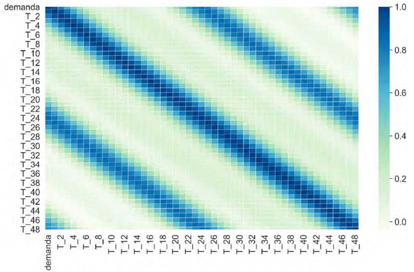
Finally, from in each of the scenarios, new features were generated from datasets associated with past demand measures to train the models. In particular, the last 48 measures were considered for each record to capture at least two days of consumption pattern directly in the features.
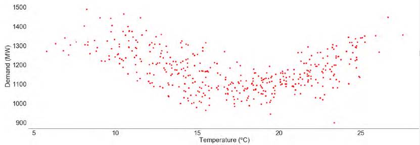
Several visualization analysis were performed to gain an intuitive insight of the information contained in each feature. The most relevant fact confirmed in this preliminary analysis was the daily periodicity of the demand value in all scenarios. The diagram shown in Figure 1 reports the high correlation between actual demand and the demand of the same hour of two days before in the case of the industrial park scenario. Weather data was not considered in the industrial scenario because of the very low correlation. However, in both scenarios that contain residential consumption data, weather variables are highly correlated with demand. Figure 2 presents the relation between temperature and total consumption for the scenario of total demand of Uruguay showing that demand values are higher in extreme temperatures. Data preprocessing was performed using pandas library[32]. A linear regression model M sim was trained using the sklearn toolkit[33], configured with default parameters as benchmark model. New training and test datasets were produced keeping only the relevant features, according to the analysis performed to determine the relative importance of each feature.
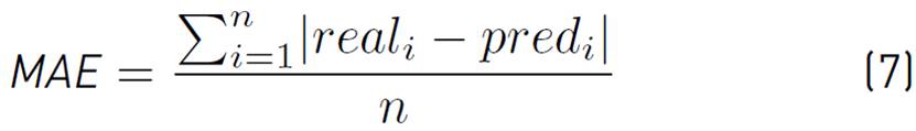
Metrics. Three standard metrics were used for evaluation: Mean absolute percentage error (MAPE, Equation (5)], root mean square error (RMSE, Equation (6)] and mean absolute error (MAE, Equation (7)]; real i represents the measured value for t = i, pred i represents the predicted value and n represents the predicted horizon length.


Training the one hour ahead forecasting models
Once all data were prepared for model training, a four-step procedure was applied for training and evaluation in all the scenarios studied. The four steps are:
Training and test sets were generated in a 3:1 proportion. In the industrial park scenario, the training set considered data from 2014 to 2016 and the test set considered data from 2017. In the substation scenario, the training set considered data from January 2017 to June 2018 and the test set from July 2018 to December 2018. In the total demand scenario, the training set uses data from 2010 to 2016 and the test set considered data from 2017 to 2018.
A simple base model was trained for benchmarking. Using the trained model, a recursive feature elimination process was performed. The ten most important features are preserved.
Several models were trained and compared with the benchmark model.
The best model according to MAPE metric was chosen.
An optimization of hyperparameters of the best model was performed using grid search techniques.
Finally, the best model found with the optimized hyperparameters was used as a reference to train the 24 hour forecasting model.
Generation of the 24 hour model
The best model configured with the best hyperparameters obtained in the previous step, was used to generate twenty four modelsM1,M2, ...,M24 to forecast day ahead hours. The twenty four models were generated by applying the following procedure:
Training and test sets were generated using the same procedure described in Section 3.1. In the industrial park scenario, the training set considered data from 2014 to 2016 and the test set considered data from 2017. In the substation scenario, the training set considered data from January 2017 to June 2018 and the test set from July 2018 to December 2018. In the total demand scenario, the training set uses data from 2010 to 2016 and the test set considered data from 2017 to 2018.
Model Mi was trained using yi as output, where yi consists of the demand value corresponding to i hours ahead, and input X is enriched for models M i , i > 2 with a new column consisting of the i − 1 prediction obtained by the trained model M i−1
Models M i are assembled to get a complete model M to forecast the next 24 hours altogether.
3.2 Implementation
This section describes the implementation of the approach described in Section 3.1.
Computational platform and software
The experimental evaluation was performed in an HP ProLiant DL380 G9 high end server with two Intel Xeon Gold 6138 processors (20 cores each) and 128 GB RAM, from the high performance computing infrastructure of National Supercomputing Center, Uruguay (Cluster-UY)[34].
The proposed approach was implemented in Python. Several scientific packages were used to handle data, train models and visualize results. Used packages included pandas, sklearn, and keras.
A generic module was implemented to train various type of models following a pipeline processing. Parameter tuning of the studied models were performed using RandomizedSearchCV and GridSearchCV modules from sklearn. The main details of the implementation of the studied models are provided in the following subsections.
Implementation of one-hour model
All one hour models described in this section use training and test sets and data preprocessing presented in Section 3.1.
Base model: Linear regression. A linear regression model was trained to be used as a baseline for the results comparison. A recursive feature selection strategy[35] was also applied on this model for each of the three scenarios to determine the most important features.
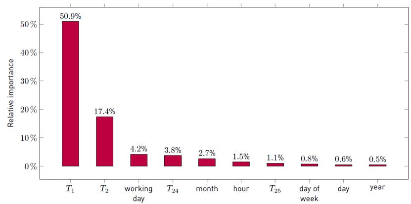
The rest of features were removed from the dataset. Ten features were selected based on their relative importance in the industrial demand scenario:
T 1, T 2, T 24, T 25: demand values lagged.
workingday: flag indicating whether the day of measured value is a working day
month: month on which the measure was taken.
hour: hour of the day on which the measure was taken.
dayofweek: day of the week on which the measure was taken.
day: day of month on which the measure was taken.
year: year on which the measure was taken.
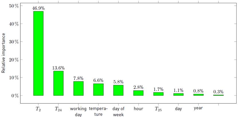
For the two residential scenarios, the ten most important features were:
T 1, T 2, T 24, T 25: demand values lagged.
temperature forecast: temperature external forecast for the hour to be considered.
workingday: flag indicating whether the day of measured value is a working day
month: month on which the measure was taken.
hour: hour of the day on which the measure was taken.
dayofweek: day of the week on which the measure was taken.
year: year on which the measure was taken.
The most relevant past demand values are T 1, T 2, T 24, and T 25 because the current demand is highly correlated with the immediate past demands and also with the demands of the previous day at the same time, due to the daily periodicity. It is worth noting that temperature is the fifth most important feature in scenarios that involve residential demand, in spite of being excluded of the industrial model due to the very low correlation with demand in that case. When training hourly models, temperature external forecast is considered for the corresponding hour.
The full analysis of feature selection experiments is presented and discussed in Section 4.1.
Selection of the best method. Seven regression models were trained for each scenario, including the base model considering the ten most important features and default parameters. The studied models included trained using the scikit-learn API[36]:
Linear Regression, MLP, Extra Trees, Gradient Boosting, Random Forest, K-Neighobors and Ridge.
These models were evaluated using the MAPE metric and the linear regression model was used to determine a baseline performance value. The most accurate method was chosen for further evaluation (this method is called M best ).
Optimization of the best method. Parameter search techniques were applied for each scenario to optimize a model based on the best method obtained (M best ). The model M best trained with default parameters was optimized using two standard tools available in scikit-learn:
GridSearchCV: combines an estimator with a grid search preamble to tune hyper-parameters. The method picks the optimal parameter from the grid search and uses it with the estimator selected according to a predetermined metric.
RandomizedSearchCV: sets up a grid of hyperparameter values and selects random combinations to train the model and score. After that, the method finds the best parameters setting according to a predetermined metric.
The best parameter set obtained for M best are used in an optimal model M opt . The main details of the implementation of the complete model are described in the next subsection.
3.3 Implementation of the complete model
Model Mopt was optimized for predicting the next hour and used for predicting any of the following 24 hours to build the complete model. This decision was adopted assuming that the forecasting quality of the parameter setting obtained in the previous phase is independent of the hour used as output.
To build the complete model, 24 instances of the optimized model M opt were trained. These instances are called Mopt,i , defining the model trained to forecast the i th hour ahead. The output yi used to train the model consisted of the demand value for the i-th hour ahead.
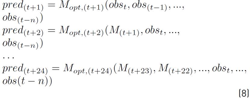
For i > 2, the input X i is enriched with a new set of columns consisting in all predictions obtained by models M opt,1 , ...,M opt,i−1 . Then, the complete solution uses a different model for each time step to predict. Predictions for previous time steps are used as input for the prediction on the following time step.
This way, a hybrid strategy is applied to M opt , described in Equation (8).
Finally, the complete model M opt is computed by Equation (9). The output of the model is a 24 valued vector, one prediction for each hour.

4. Experimental analysis
This section presents the results of the experimental analysis of the proposed computational intelligence methods for day ahead electricity demand forecasting in industrial and residential scenarios.
4.1 Recursive feature elimination
A feature selection analysis was performed using the recursive feature elimination tool available in sklearn.
A model is specified and a number of features are selected, and the tool works by recursively removing features and building a new model (of the specified type) on those remaining features.
The accuracy of the new model is used to identify the features or combination of features that contribute the most to predicting the target attribute.
The recursive feature selection tool was applied over the linear regression method described in Subsection 3.2 in each of the three scenarios, to study up to ten features.
Figure 3, 4 and 5 summarize the main results of the analysis, reporting the relative importance of the ten most important features for each scenario.
The most relevant conclusion of the feature selection analysis is the high relative importance of temperature in both scenarios related with residential demand. This is a expected result due to the high incidence of temperatura on residential energy consumption, in contrast to its low incidence on industrial energy consumption.
4.2 Experimental results on preliminary models
Performance metrics defined in Section 3.1 were used to evaluate the implementation of the one hour models as described in Section 3.2.
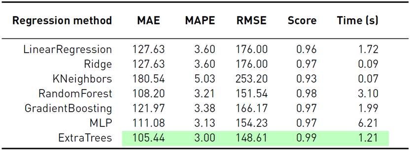
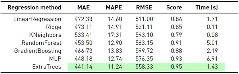
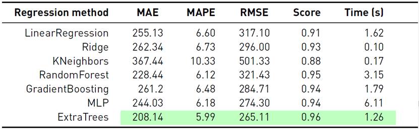
Tables 1-3 report the obtained results of the studied forecasting models for each scenario. The best results are reported in cells with green background.
Results reported in Table 1 for the industrial scenario indicate that three of the studied methods achieved the best results regarding the analyzed metrics. Focusing on MAPE, Extratreesregressor improved over MLP by 4.16% and over RandomForest by 6.54%.
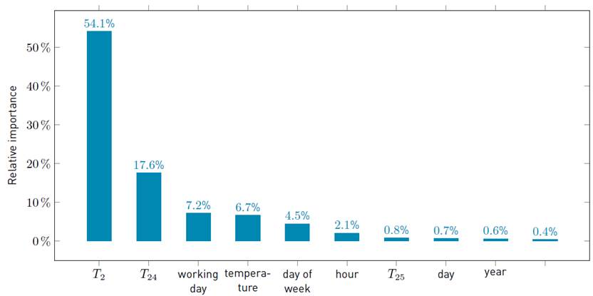
Figure 5 Relative importance of most important features (percentage values), total demand of Uruguay
In turn, results reported in Table 2 for the substation scenario and in Table 3 for the total demand scenario indicate that Extratreesregressor was also the best model in both cases. Additionally, in all scenarios the training time of Extratreesregressor was approximately three times shorter than RandomForest and six times smaller than MLP.
Overall, ExtraTreesRegressor was the most effective model for forecasting the next hour, outperforming all the other methods regarding the three standard metrics studied in each scenario. According to these results, ExtraTrees was selected as the best method for showing the best performance and a low training time. Thus, in following sectionsM best = ExtraTreesRegressor.
4.3 Parameter tuning
Parameter tuning techniques described in Section 3.2 were applied on the best modelM best .
The input for both grid search studied techniques in the three data scenarios was generated using the following values:
n_estimators: [10, 50, 75, 100, 150];
max_features: [auto, sqrt, log2];
max_depth: [50, 100,150, 200, 250]
GridSearchCV achieved the best results with the same parameters setting for all scenarios. The best parameter setting found by the algorithm was n_estimators=50, max_features=auto and max_depth=250.
Regarding MAPE metric, results computed using the best configuration significantly outperformed results of the second best configuration: improvements were 14% for the industrial demand scenario, 11% in the substation demand scenario, and 12% in the total demand scenario.
4.4 Experimental results after parameter tuning
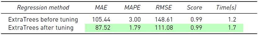
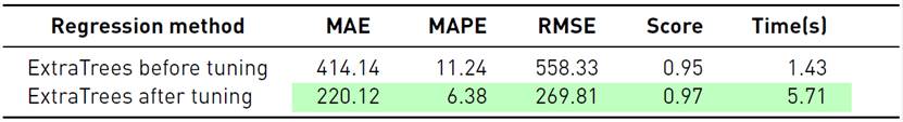
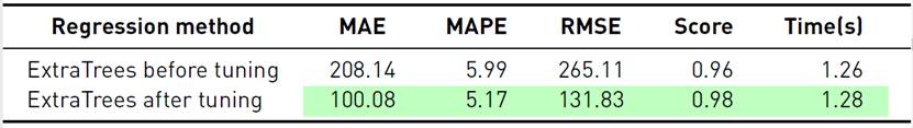
Tables 4-6 report the results of the ExtraTreesRegressor model before and after parameter tuning for each scenario. The best results are highlighted (cells with green background).
Results computed by the tuned configuration of ExtraTreesRegressor considerably improved the baseline (non-tuned) version, regarding the three studied metrics. In particular, MAPE reduced from 3.00% to 1.79%.
The performance improvement just demanded a negligible increase on training time increases after parameter tuning from 1.2 s to 1.7 s.
5. Experimental results of the complete model
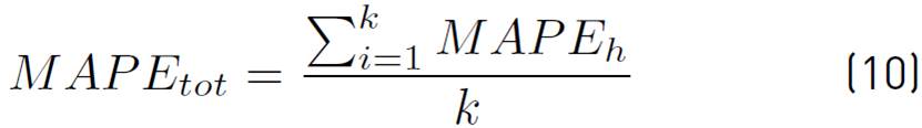
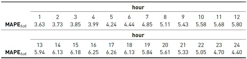
The forecast accuracy of the final model was validated by applying MAPEtot a metric that extends M APE . Let
MAPE h be the MAPE value for a predicted horizon h, the extension of MAPE to the complete testing set is defined by Equation (10).
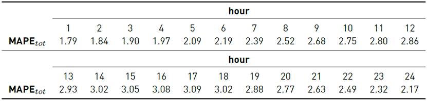
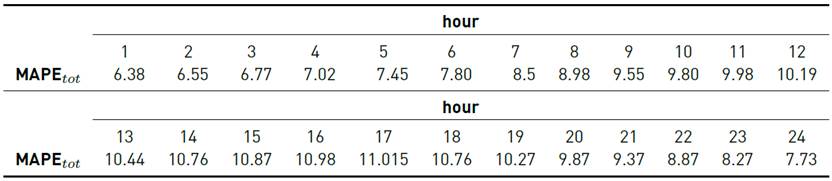
Tables 7-9 report the results for each one of the 24 models.
The expected behaviour is that the models trained for highly correlated hours in the future respect to the current hour, perform better than less correlated.
This fact is due to predictability, and it is enhanced when the correlation between input features and predicted values is higher.
According to Figure 1, highly correlated demand values correspond to the immediately preceding hours and from the same hours of the day before.
Analyzing the obtained results for the MAPE tot metric for each one of the 24 hourly models, the performance got worse from i = 1 to 17 and then improved from i = 18 to 24. These results show that highly correlated demand values performed better, as expected.
Finally, the complete model ET opt was applied. A day-ahead hourly forecast demand curve was generated for each time window for the testing set and the MAPE tot value was calculated.
The final result for the complete model was MAPE tot = 2.55% in the industrial scenario, MAPE tot = 5.17% in the industrial scenario and MAPE tot = 9.09% in the substation scenario.
These results imply that the model obtained for the day ahead demand forecasting of the industrial park analyzed incurs in an error that is considered very low for most of the studies that rely on these types of models[5, 6].
For the substation scenario, there are no known previous analysis in Uruguay to compare, but considering that the group of homes connected to the substation is small, an error of MAPE tot = 9.09% is considered acceptable.
For the total demand scenario, a relevant baseline for comparison is provided by the prediction models currently used by the National Administration of the Electric Market, Uruguay (ADME, adme.com.uy). According to public information reported in the ADME website, currently used prediction models have errors (MAPE tot ) between 5.00% and 7.00%, with an average of MAPE tot = 5.52%. The model evaluated in this article reported an error of MAPE tot = 5.17%, which constitutes an excellent result, improving over baseline ADME methods by 6.34%. This is a very encouraging result for total demand prediction in Uruguay.
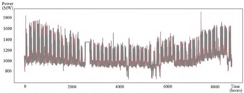
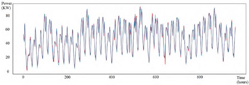
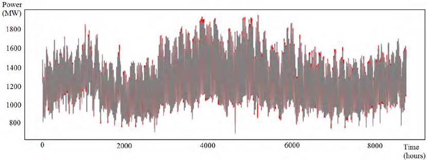
Figures 6-8 present samples of the real demand curve and the predicted demand curve using the best model, for a subset of the testing set considered in the experiments. For the industrial demand scenario, the presented subset corresponds to the complete data from year 2017. For the substation scenario prediction, data from September 1 st , 2019 to December 10 th , 2019 are used. Finally, for the total demand scenario the subset is the complete data from year 2018.
The scenarios analyzed are representative of the studied industrial and residential demands. The results obtained with the model created were very good for all three cases.
6. Conclusions and future work
This article presented an approach to address the problema of day ahead electricity demand forecasting.
Several machine learning models were presented and studied for next hour forecasting. Recursive feature selection was applied to select the most relevant features to train the studied models. After a comparative evaluation, the best model was optimized using random search and grid search techniques.
A hybrid strategy (combining direct and recursive approaches) was built based on the optimized model for single hour prediction. It was applied to build a complete day ahead electricity demand hourly forecasting model in three scenarios: an industrial demand forecasting scenario in Spain, a residential demand forecasting scenario for a substation in Montevideo, and a total demand forecasting scenario of Uruguay, including both residential and industrial consumers.
The experimental evaluation was performed considering data from January 1 st , 2010 to December, 10 th , 2019. An extension of the MAPE metric was used to evaluate the complete model for the three scenarios using testing sets.
For the industrial demand scenario, the evaluation of the complete model reported a value of MAPE tot = 2.55%. This is a very effective prediction result, which indicates that the proposed algorithm is effective for addressing the problem of day-ahead industrial demand forecasting, despite of using a model that do not consider weather variables.
For the substation scenario, the evaluation of the complete model reported a value of MAPE tot = 9.09%. In this case, the proposed algorithm considered weather variables due to the high correlation detected between them and electricity demand. Results indicated that the complete model can predict the demand with an aceptable accuracy, in line with results from the literature, especially considering that the variation of residential demand of a small group of houses is significantly higher than the variation of industrial demand.
Finally, the application of the complete model to the total demand scenario in Uruguay reported a value of MAPE tot = 5.17%. In this scenario, only one weather variable (temperature) was considered (humidity and wind speed were excluded due to low relative importance).
Results obtained are very promising considering that the models currently used in Uruguay, from the National Administration of the Electric Market has a MAPE tot error between 5.00% and 7.00%.
The main lines for future work are related to consider deep learning techniques (e.g., recurrent/long-short term memory neural networks) for enhancing the prediction, since they can provide accurate results in scenarios that are difficult for other simpler methods, i.e. when handling large volumes of historical data. These techniques have been successfully applied to forecasting problems with complex state structures in explanatory variables, so they can be useful tools to deal with uncertainty in electricity demand.
Another line of future work consists in enriching the studied models to generate mid-term and long-term synthetic demand scenarios that preserve the statistical structure of historical data. These kinds of models are very relevant to be included in planning and operation models based on new computational intelligence techniques such as reinforcement learning or approximate dynamic programming. Furthermore, prediction results can be applied in practice for household energy planning by using intelligent recommendation systems[37].

