English (pdf)
 Article in xml format
 Article references
 Send this article by e-mail
 Cited by SciELO
  Cited by Google
  Similars in
SciELO
Similars in
SciELO  Similars in Google
 Permalink
1. Introduction
The behavior of beam-column elements resting on elastic foundations has been a subject of great interest in the last century [e.g.,[1-8]]. It has practical applications in civil engineering and other related engineering fields. Winkler[1], one of the pioneers in the field, proposed to represent the soil as a series of closely spaced linear springs. This idealization, currently known as the Winkler approach, though practical, is a simplification of the soil medium because it neglects the shear interaction between the elements. To overcome this limitation, several authors have proposed the use of a two-parameter model, where the first parameter is analogous to the Winkler’s spring and the second one represents a shear layer connecting the springs at the top ends[9-11]. Some models are derived to account for a uniform distribution of the modulus of subgrade reaction (i.e., homogeneous soil). In this case, the DE governing the response of the element can be readily solved using classical approaches. However, when the soil parameter varies along the element (i.e., non-homogeneous soil), the DE has non-constant coefficients, and its solution becomes difficult. Thus, in some cases it cannot be solved analytically and a numerical solution needs to be provided. The DTM is used to solve the governing differential equation, and its corresponding boundary conditions. The DTM is a simple, efficient, and powerful method that converts differential equations into recursive algebraic expressions [e.g.,[12-14]]. The DTM was first implemented by Zhou [15] to solve electrical circuit problems, and it is a practical and powerfully approach to solve linear and non linear differential equations. Some researchers have successfully employed the DTM to conduct static and dynamic analyses of beam-column elements [e.g.,[16-22]], but, in general, its application to civil engineering related problems is limited when compared to other fields. The following conditions are incorporated in the proposed analysis: (a) a Pasternak two-parameter elastic foundation to account for the interaction between the springs; (b) an external transverse load acting on the element that fits a quadratic function. (i.e., offers flexibility to consider uniformly distributed, trapezoidal or parabolic transverse loads); (c) any axial load, horizontal load and moment at each end of the element; and (d) semirigid connections and lateral restraints at the ends of the element. Both static and stability analyses can be conducted using the same set of equations, and the effects of any end-boundary condition on the element response can be studied without the need to discretize the solution for each individual boundary condition.
2. Structural Model
2.1 Assumptions
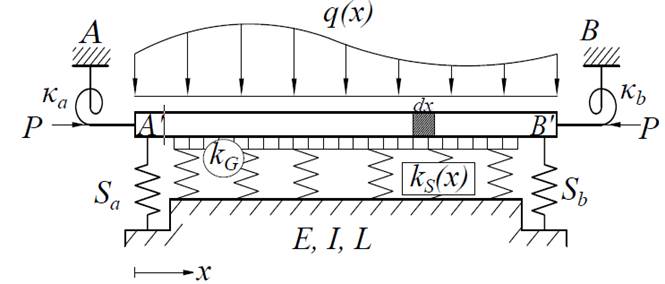
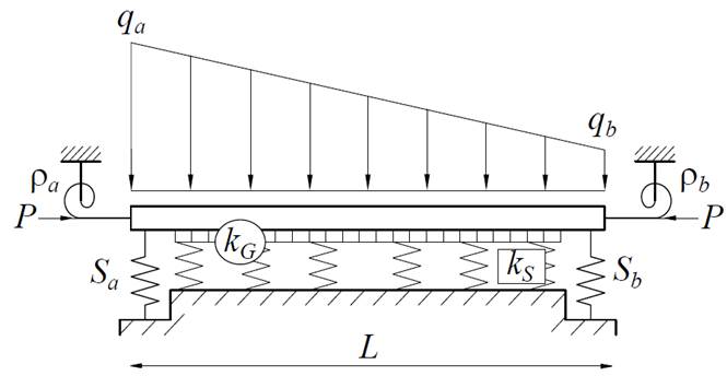
The proposed model considers a beam-column element A′B′ connected at both ends A and B as shown in
Figure 1 by elastic springs AA′ and BB′ with flexural connectors κ a and κ b (units in force × distance/radian) and lateral springs S a and S b (units in force/distance). It is assumed that the beam-column A′B′ is: (1) prismatic with constant cross-sectional area, moment of inertia I about the principal axis, and span L; (2) made of a linear elastic, homogeneous and isotropic material with elastic moduli E; (3) resting on a two-parameter elastic foundation, where the first parameter (i.e., k s ) can be either constant (homogeneous soil) or vary linearly with length or depth (non-homogeneous soil); and (4) subjected to an axial load P (tension or compression), horizontal load V and moment M at its ends. It is assumed that all transverse deflections, rotations and strains along the beam are small so that the principle of superposition is applicable. For convenience, fixity factors parameters ρa and ρb are introduced. ρa = 1/(1 + (3EI/L)/κ a ) and ρb = 1/(1 + (3EI/L)/κ b . These factors vary from zero (perfectly hinged connection) to one (clamped connection)[23].
2.2 Governing Equations
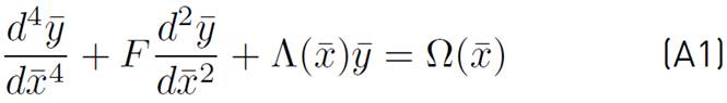
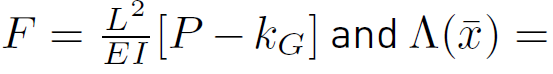
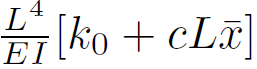
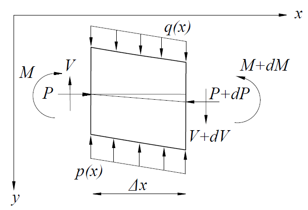
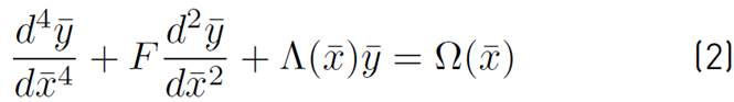
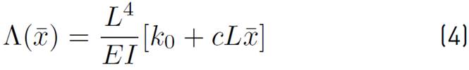
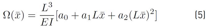
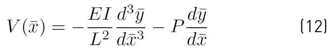
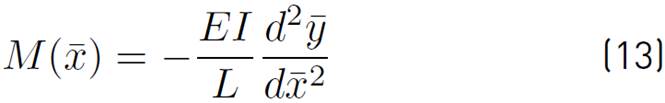
The governing DE of the beam-column element described in Figure 1 is obtained by applying equilibrium to the free-body diagram shown in Figure 2[24]. The DE is described by Equation (1) as follows:
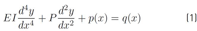
where
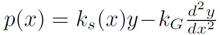 is the reaction normal to the element and q(x) is an external transverse load that fits a second-degree polynomial function [i.e., q(x) = a
0+a
1
x+ a
2
x
2]. k
s
(x) = k
0+cx is the modulus of subgrade reaction (first-parameter) and k
G
is the shear layer connecting the elements at the top ends (second-parameter). Introducing
is the reaction normal to the element and q(x) is an external transverse load that fits a second-degree polynomial function [i.e., q(x) = a
0+a
1
x+ a
2
x
2]. k
s
(x) = k
0+cx is the modulus of subgrade reaction (first-parameter) and k
G
is the shear layer connecting the elements at the top ends (second-parameter). Introducing
the non-dimensional expressions
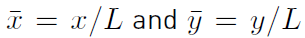 into Equation (1) yields to Equation (2):
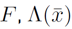
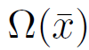
where
 , and
, and
 are given by Equations (3) - (5):
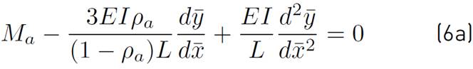
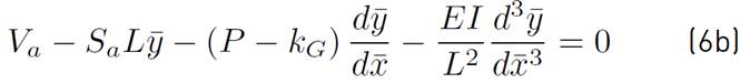
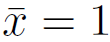
The boundary conditions at
 are expressed by Equations (6a) - (6b):
and at
 by Equations (6c) - (6d):
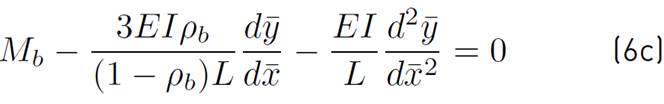
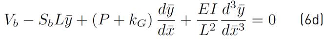
where V a , V b ,M a ,M b are the horizontal load and bending moment applied at ends A and B, respectively. Equation (2) is the normalized fourth-order linear differential equation with non-constant coefficients that describes the behavior of the proposed beam-column. Equations (6a)-(6d) are the corresponding boundary conditions of the DE.
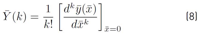
2.3 Differential transformation method
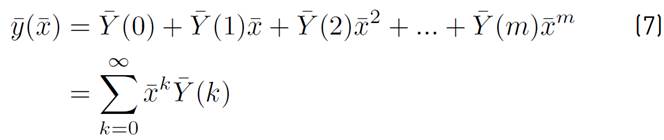
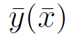
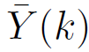
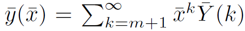
The DTM is an analytical approach to solve differential equations. It is based on Taylor series, where the dependent variable is expressed as a series of infinite terms of the independent variable. The advantage of the DTM over other conventional approaches is that the problem is reduced to solve a system of two linear algebraic equations, which solution is easy to implement in a computational software or a personal calculator. Using conventional approaches, the mathematical formulation and solution of the proposed structural model becomes cumbersome and tedious to implement. The solution to the DE is:
where
 is the original function (i.e., transverse deformation) and
 is the transformed expression of the k
th coefficient given by Equation (8).
is the transformed expression of the k
th coefficient given by Equation (8).
In practice, function
 in Equation (7) is expressed as a finite series of order m, so that
 is small.
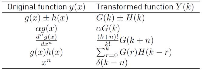
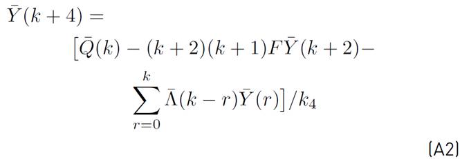
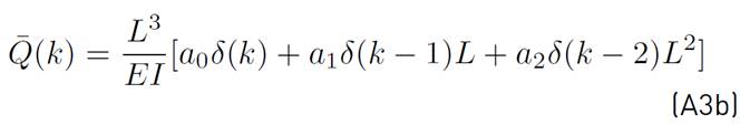
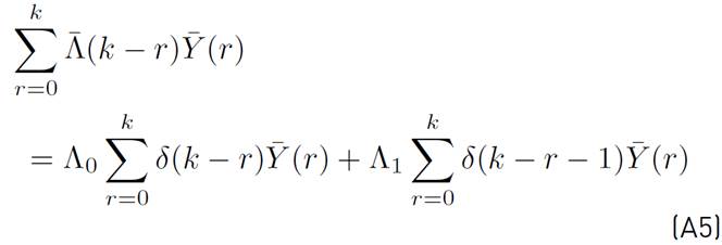
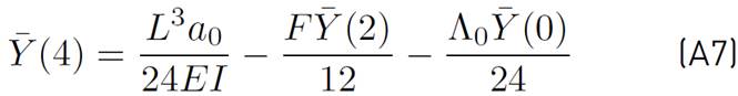
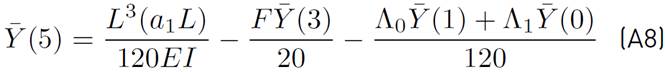
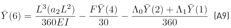
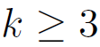
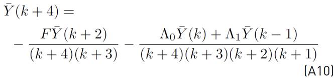
Substituting the transformed functions shown in Table 1 into Equation (2), the following recurring form of the DE is obtained (see Equations (A1)-(A10) from appendix A):
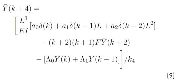
where k
4 = (k +4)(k +3)(k +2)(k +1),
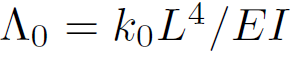 and
and
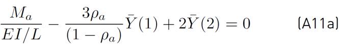
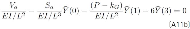
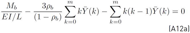
 . Using Equation (7), the boundary conditions (i.e., Equations (6c) and (6d)) are transformed as (see Equations (A12a)-(A12b) from appendix A]:
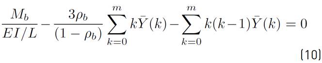
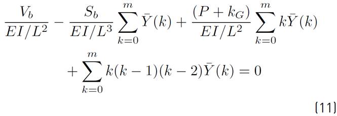
Equations (10) and (11) are a system of two linear algebraic equations in terms of
 and
and
 (i.e., deflection and rotation at
 ). Terms
 and
and
 are found from Equations (A11a) and (A11b), respectively. The other terms,
 , are found from the recurrence equation (Equation (9)]. To solve the system, the values of
and are initially assumed, and then the other terms of the series are determined. The intersection between these two lines is the solution
and
that satisfies both boundaries conditions (i.e.,
, are found from the recurrence equation (Equation (9)]. To solve the system, the values of
and are initially assumed, and then the other terms of the series are determined. The intersection between these two lines is the solution
and
that satisfies both boundaries conditions (i.e.,
 and
and
 ) Once the solution is known, coefficients
 to
to
 can be computed. The transverse deflection profile of the element is determined from Equation (7), the rotation from the first derivative of
 , and the shear force and bending moment profiles from:
3. Comprehensive examples and verification
Five examples are presented to validate the accuracy of the proposed approach. The results are compared with those obtained from other analytical approaches and finite element analyses in SAP2000[25]. In SAP2000, beam elements were chosen to model the beam-column element and the shear deformations were ignored by equaling the shear rigidity to infinity.
Example 1: Beam-column resting on a Pasternak elastic foundation.
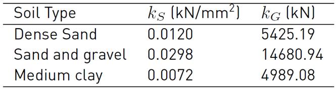
Determine the deflection, rotation, shear force, and bending moment profiles of the beam-column element resting on the Pasternak elastic foundation shown in Figure 3, and for the three different soil types listed in Table 2 (i.e., dense sand, sand and gravel, and médium clay). The beam-column element characteristics and soil types described in this example correspond to those presented by Arboleda-Monsalve et al.[26]. The beam is subjected to an axial compressive load and a trapezoidal transverse load as shown in Figure 3. Its assumed that E p = 12 kN/mm2; I p = 5.208 × 109 mm4; L = 6000 mm; ρ a = 0.7; ρ b = 0.3; S a = 15 kN/mm; S b = 25 kN/mm; and the external loads are: q a = 0.4 kN/mm; q b = 0.2 kN/mm; P = 3000 kN. Figure 4 shows the profiles of the vertical deflection, y(x), rotation, θ(x), bending moment, M(x), and shear force ,V (x), along the element. The results from the proposed approach are in excellent agreement with those obtained from SAP2000, where the element was subdivided into 50 segments to provide sufficient accuracy.
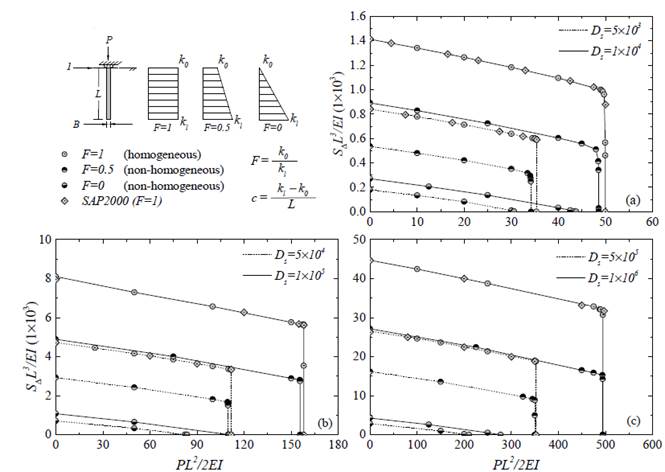
Example 2: Second-order lateral stiffness of piles in non-homogeneous soil.
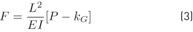
The variation of the pile lateral stiffness with changes in axial load and different distributions of the modulus of subgrade reaction (k
s
) is presented. Let F = k
0
/k
l
be a non-dimensional term relating the modulus of subgrade reaction at
 and
and
 . Then, F = 1 represents a homogeneous soil (uniform distribution) and
 a non-homogeneous soil (linear distribution). Although any end-boundary condition maybe analyzed with the proposed formulation, for the sake of brevity, only piles free at the bottom and rotational inhibited at the top (ρ
a
= 1) are investigated. This condition is encountered in practice in the analysis of pile-supported wharves and piers[27]. The lateral stiffness index is defined as
a non-homogeneous soil (linear distribution). Although any end-boundary condition maybe analyzed with the proposed formulation, for the sake of brevity, only piles free at the bottom and rotational inhibited at the top (ρ
a
= 1) are investigated. This condition is encountered in practice in the analysis of pile-supported wharves and piers[27]. The lateral stiffness index is defined as
 , where
 is the lateral stiffness of the pile. The axial load and lateral stiffness indices are defined as N = PL
2
/2EI and D
s
= klL
4
/EI, respectively. The lateral stiffness,
is the lateral stiffness of the pile. The axial load and lateral stiffness indices are defined as N = PL
2
/2EI and D
s
= klL
4
/EI, respectively. The lateral stiffness,
 , associated to each axial load is computed by imposing a horizontal unit load (Va = 1) and determining the transverse displacement at the top of the element. Figure 5 shows the results from the parametric study. It is noted that,
 is the greatest for the uniform distribution of k
s
and the lowest for the linear triangular distribution. This highlights the importance of the upper portion of the soil on the pile lateral stiffness. When F = 1 and F = 0.5,
decreases linearly as the axial load increases, and it drops almost to zero when the axial load approaches to the critical load. For the case when F = 0 (i.e., linear variation of k
s
) the variation of
is almost linear over the whole range of axial loads. The results are in agreement with those obtained from SAP2000 (for F = 1).
is the greatest for the uniform distribution of k
s
and the lowest for the linear triangular distribution. This highlights the importance of the upper portion of the soil on the pile lateral stiffness. When F = 1 and F = 0.5,
decreases linearly as the axial load increases, and it drops almost to zero when the axial load approaches to the critical load. For the case when F = 0 (i.e., linear variation of k
s
) the variation of
is almost linear over the whole range of axial loads. The results are in agreement with those obtained from SAP2000 (for F = 1).
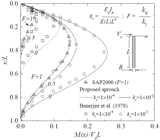
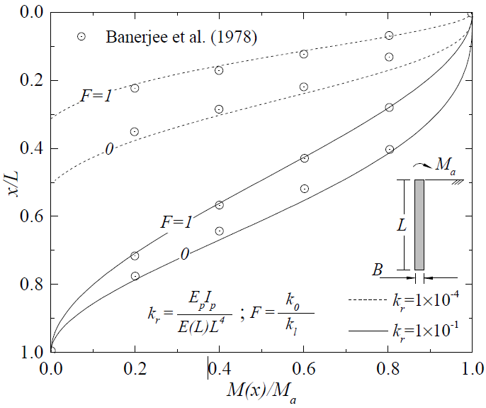
Example 3: Bending moment profile of a laterally loaded pile.
The proposed method captures the complete normalized bending moment profile of laterally loaded piles. The results are compared with those obtained from the numerical approach proposed by Banerjee and Davies[28]. The pile has a slenderness ratio of L/B = 25, and it is fully embedded in homogeneous or non-homogeneous soil represented by values of F = 1, F = 0.5, and F = 0. The analysis was conducted for a free-free pile. Banerjee and Davies[28] defined the non-dimensional expression for the relative pile flexibility ratio as k r = E p I p /E(L)L4. Note that k r = 1 × 10⁻¹ corresponds to a very stiff pile (i.e., short pile) and k r = 1 × 10 −4 to a flexible pile.
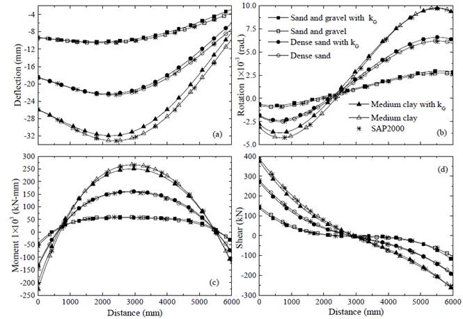
Figure 4 Example 1: (a) deflection; (b) rotation; (c) bending moment; (d) shear force of the beam-column element.
Figures 6 and 7 show, respectively, the normalized bending moment distribution of the pile when subjected to a horizontal load and a bending moment at the pile head. The results show that, regardless of the pile slenderness ratio, both the moment distribution and location of máximum moment are significantly affected by the variation of k s . Overall, bending moments are greater in short piles tan in flexible piles, and the magnitude decreases as k s moves from a linear triangular variation toward a uniform variation. The results are in good agreement with those reported by Banerjee and Davies[28] and computed with FE approaches (for the case of F = 1).
Example 4: Lateral deflection of short and long piles.
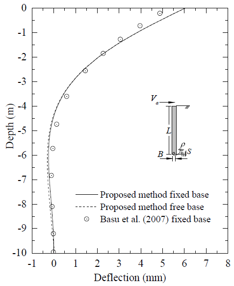
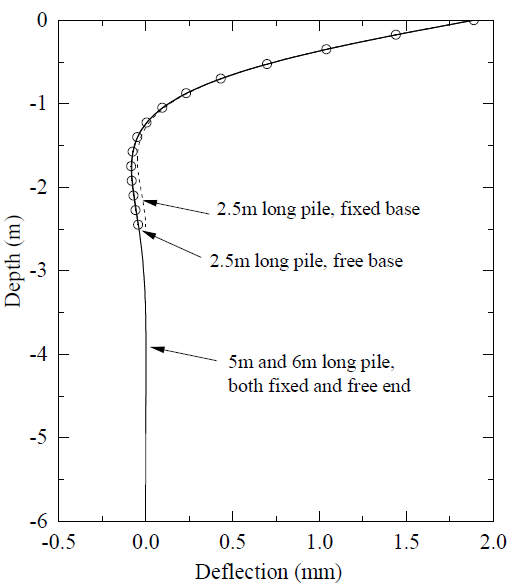
When subjected to external lateral loads, short piles experience a rigid body translation and rotation, and therefore their response is influenced by both end-boundary conditions. On the other hand, long piles are those whose response is not influenced by the boundary condition at the base[29]. In general, a long pile is considered a pile with a slenderness ratio (L/r > 80). Piles with L/r < 80 exhibit a transition from a flexible behavior toward a rigid one[30]. Pile slenderness ratio (L/r) and relative stiffness ratio (E p /k s ) have a strong influence on the pile response. Here, some examples are reproduced from Basu and Salgado[31] to show this particular behavior. Figure 8 shows the deflection profile of a concrete short pile with radius r = 0.5 m, Length L = 10 m, and modulus of elasticity E p = 2.4 × 10⁶ kPa, fully embedded in a clay deposit with k s = 11.6 MPa and k G = 6.8 MN, and subjected to horizontal load of 100 kN at the head. The pile is considered to be free at the head (ρ a = 0 and S a = 0) and either free (ρ b = 0 and S b = 0) or fixed (ρ a = 1 and S b = ∞) at the bottom. The results obtained from the proposed method and the method of initial parameters (MIP) developed by Basu and Salgado[31] show good agreement. Figure 9 shows the transverse deflection of a concrete pile with radius r = 0.25 m and lengths of L = 2.5 m, L = 5 m, and L = 6 m, embedded in a dense sand deposit with k s = 130 MPa and k G = 7.9 MN, and subjected to a horizontal load of 100 kN at the head. The pile is considered to be free at the head and either free or fixed at the bottom. The 2.5m long pile shows that the base condition influences the deflection response. Meanwhile, the 5 m and 6 m long pile have the same response for both free and fixed conditions.
Example 5: Normalized free-head pile displacement in homogeneous soil
Higgins et al.[30] used FEM analysis coupled with Fourier techniques to estimate lateral deflections and máximum moments of laterally loaded piles. Higgins et al. Classified the pile depending on its relative stiffness (E p /k s ) and slenderness ratio (L/r). A flexible long pile depends only on its relative stiffness, a flexible short pile on both relative stiffness and slenderness ratio, and a rigid pile only on its slenderness ratio. Figure 10 shows the normalized free-head pile deflection in homogeneous soil when the pile head is subjected to a horizontal load or bending moment. From this figure it is noted that, for flexible long piles, the head deflection decreases as the relative stiffness increases, and the decrements become less pronounced as the pile stiffness ratio increases. This response is more evident in piles with low values of soil stiffness ratios, where the lateral deflection becomes almost constant after a certain value of slenderness ratio.
4. Conclusions
A simple analytical approach to study the behavior of beam-column elements on homogeneous or non-homogeneous soil was presented and discussed. The fourth-order order DE with non-constant coefficients was solved using the differential transformation method (DTM). The solution to this DE using conventional approaches is rather complex. However, when the DTM is used, the resulting expressions consist of two linear algebraic equations which solution is easy to code in any computational software or spreadsheet. The same set of equations can be used to conduct either static or stability analyses of beam-column elements. The effects of various slenderness ratios, pile-soil stiffness ratios, and classical and semi-rigid boundary conditions can be easily studied with the proposed formulation. Five examples were presented to validate the accuracy and simplicity of the approach as well as its applicability over a wide range of practical applications. The results from the proposed model were in good agreement with those from FE analysis and other methods available in the technical literature.
As potential future studies, the proposed formulation can be extended to investigate i) the effect of an initial deformation on the beam-column response, b) cracked beam-columns by modeling the cracks as rotational springs, ii) static, elastic stability, and dynamic analysis of piles partially embedded in a multilayered soil by finding the static and dynamic stiffness matrices and corresponding loading vector, among others.