


 Inglês (pdf)
 Artigo em XML
 Referências do artigo
 Enviar este artigo por email
 Citado por SciELO
  Citado por Google
  Similares em
SciELO
Similares em
SciELO  Similares em Google
 Permalink
1. Introduction
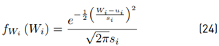
The normal distribution is the most common probability distribution function (PDF) used in any scientific field if we want to characterize a random variable (RV). This occurs because many natural phenomena are modeled according to the central limit theorem. Sometimes, random variable values are pretty small, and it is necessary to expand those values through an exponential function, which is also useful for analytic treatments. Due to this, the lognormal random variable arises. It means that if we characterize a RV as X ∼ Normal [m, s] with mean m and standard deviation s, and then we calculate x = 10X , we will yield x ∼ lognormal [µ, σ] with mean µ and standard deviation σ, where: µ = κ · m, σ = κ · s and

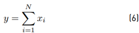
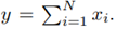
Several works shown in [1,2] have suggested that the sum of lognormal RVs can be approximated by a lognormal distribution. It means that for:

If we have N RVs
Then:

Now, through two examples, we will show whether or not in a telecommunications scenario known as characterization of the aggregate interference with N interferents, it is possible to approximate the sum of lognormal variables with a lognormal PDF.
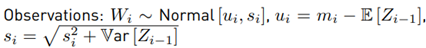
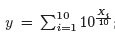
Explanation of Monte Carlo simulations 1 and 2 We’ll consider a scenario where N = 5 is the number of random variables to sum. 104 samples are generated for each of the five RVs Xi, i = [1, .., 5] using a Normal distribution function with parameters randomly selected within the range of an interference signal where m = [−80, −60] , and s = [4, 12]. The parameters selected for the mean value and variance were m = {−63, −61, −78, −61, −67}, s = {4, 5, 7, 9, 9} respectively. Then the following operation is performed:
 and finally we calculate
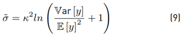
Since it has been said that y follows a lognormal PDF, then Y should have a Normal PDF. Experimentally, the mean value µ˜, variance σ˜2 and standard deviation σ˜ are obtained using the mean, var and std commands of the software Matlab. With these parameters, we generate a normal analytical PDF to compare it against the histogram of the simulation.
Simulation 2 used the following parameters m = {−74 − 60 − 76 − 69 − 71}, s = {6, 6, 5, 7, 7}. As a result of the simulations, Figure 1 shows that for N = 5, sometimes this approximation could work, but even with a small set of variables, this approximation fails.
In this way, we show two examples where there is not a straightforward method to find an approximated PDF that fits in all cases to the real PDF of the sum of lognormal variables. This wide-used approximation must be carefully handled because of the statement mentioned above; although, it is frequently used in telecommunications [1]. Our work will focus only on an efficient method to find the mean value and the variance of the sum of lognormal RV within a wide range of parameters.
The rest of this paper is organized as follows. In section II we give a background and show previous works about the sum of lognormal variables, we review some of the approximation methods and assess their accuracy. In section III, we propose a new method for computing the sum of lognormal random variables and provide equations to calculate the mean value and variance of the sum. We validate our method in section IV and finally, in section V the conclusions are given.
2. Background and previous work
Some papers such as [1,3,4] show a summary of several works that address the sum of lognormal variables. From them, we can say that the main problem with this kind of RV is due to the fact that it has neither a characteristic function nor a moment-generating function. Some works address this issue by approximating the characteristic function and obtaining either the PDF or the cumulative distribution function (CDF). However, the curve for the experimental CDF or PDF does not completely match with the analytical function [3], and their results are bounded by asymptotic tail approximations for specific scenarios. For example, in finance [5], there are simple approximations when σ tends to 1.
The errors in the CDF or PDF approximations also depend on the number of RV in the sum. On the other hand, most of the analytical approximations must be solved using numerical computation, Monte Carlo simulations, recursive algorithms or other computational techniques. So, this means that all traditional methods are inefficient and impractical for problems where the lognormal parameters change dynamically.
A paper from Wilkinson in 1934 is perhaps one of the first works to approximate the sum of lognormal variables with a PDF that is also lognormal. Although this work was not published, it was first referenced in [6]. The work of [7] approximates the sum of lognormal variables to a lognormal PDF, but it is not always correct and is only useful when σ < 4 for each RV. This approach is also known as the Fenton-Wilkinson method, since both use the same mechanism to approximate the first two moments of the sum.
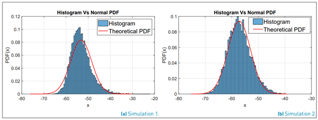
Figure 1 Comparison of the histogram of Y against an analytical Normal PDF with the parameters ˜µ, σ˜
In [8], the sum is approximated with a lognormal PDF by means of a recursive process for the calculation of the moments, but the expressions are not in closed form. In addition, it uses approximations by power series with 40 terms, which increases the computational cost. This method is useful when both the mean value and the variance of the sum are required. Then in [9] the mean value and the variance are approximated in a similar way to the work shown in [8], with the difference that the approximation is developed by a Taylor series around 0. This method is used in the area of finance. Work of [10] is based on [8], and it assumes correlated variables. A review of these approximation methods is shown in [11]. In this work, a minmax optimization approach is proposed to adjust the parameters of the lognormal PDF. This work shows that these approximations do not provide a good fit in the tails of the PDF.
A later work in [12], proposed a closed solution for the CDF, but their most relevant contribution is that they demonstrate through several results that according to the parameters used, it is not correct always to approximate the sum of lognormal variables with a lognormal PDF due to the error on the tails of the PDF function.
The work in [13] develops a closed expression to adjust the lower tail of a lognormal PDF. In [14], authors approximate the moment-generating function with a Gauss Hermite series for each variable and in [15] the authors propose an approximation of the PDF with a Log-shifted-gamma function.
[16] offers a review of related works with some focus on the approximation of the CDF for the sum of independent and correlated variables based on the characteristic function given in [17] (quadrature rules). As a result, [16] also uses the Log-shifted-gamma approximation, but it is only useful for the calculation of the CDF of the sum of 6 variables or less. Additionally, the authors propose a computational method using the Epsilon algorithm to calculate a CDF when 40 or more variables are added. In [18] the α − µ, distribution is used for the PDF, and the adjustment of parameters is done by means of a least squares regression approach. Finally, [5] approximates the PDF with a quasi-normal distribution, but this method is useful only when µ, σ ≤ 1.
2.1 Review of the approximation methods
The Fenton-Wilkinson method
One of the most widely used works for the computation of the sum of lognormal random variables is the Fenton-Wilkinson method [7] due to its good results and the simplicity of its formulas. This method states the following: a random variable X
i
follows a Normal distribution with mean mi standard deviation si. Xi ∼ Normal [mi, si], if x
i
 then: x
i
∼ lognormal [µ
i
, σ
i
]. Where: µ
i
= κ · m
i
, σ
i
= κ · s
i
and κ =
then: x
i
∼ lognormal [µ
i
, σ
i
]. Where: µ
i
= κ · m
i
, σ
i
= κ · s
i
and κ =
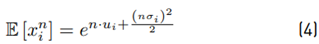
 The 1st (n = 1) and 2nd (n = 2) moments of x
i are given as:
The 1st (n = 1) and 2nd (n = 2) moments of x
i are given as:
If we have:
Assuming that y ∼ lognormal [˜µ, σ˜]. then:
Finally:
Now, if we do:

Then:

Now, we assess whether this method works correctly for the calculation of the mean value and variance through a Monte Carlo simulation.
Explanation of Monte Carlo simulation 3 used to analyze the Fenton-Wilkinson method As an example, we will use three RV’s (N=3) with 107 samples for each. X
i
, i = [1, 2, 3] follows a Normal PDF. We calculate
 to generate lognormal RV’s and
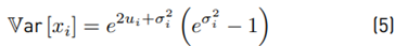
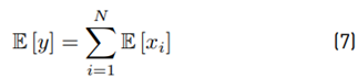
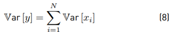
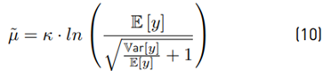
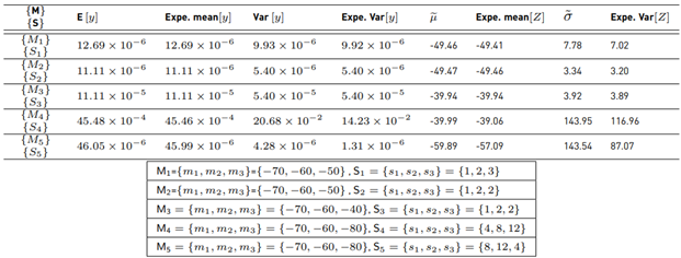
 Then, we get the experimental ˜µ, σ˜. Analytically Equations (7) and (8) are used to get E [y] and Var [y]. After that, we use Equations (9) and (10) to find the theoretical µ˜ and σ˜. We compare both experimental and analytical results with different parameters m
i
, si. Those results are shown in Table 1.
Then, we get the experimental ˜µ, σ˜. Analytically Equations (7) and (8) are used to get E [y] and Var [y]. After that, we use Equations (9) and (10) to find the theoretical µ˜ and σ˜. We compare both experimental and analytical results with different parameters m
i
, si. Those results are shown in Table 1.
Note that experimental and analytical results begin to fail when si > 4, even for only 3 RVs.
The Schwartz-Yeh method
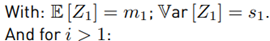
This method was proposed by [8] in 1982, which calculates the mean value E [Z] and variance Var [Z] within a set of N lognormal random variables x i ∼ lognormal [µi , σi ], i ∈ {1, 2, ..., N}. When i = 1, we have Equation (13):


With Equation (15) as:

Now, we focus on calculating the mean value.

We will use the term:
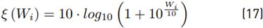
Rewritten:


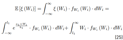
The term ξ (Wi) is originally expanded through a power series with 40 terms. After that, we calculate E [ξ] and Var [ξ]. Equation (14) shows that this method is recursive, and we have to expand this term ξ (Wi) in each i iteration which reduces the computational performance.
3. Proposed method
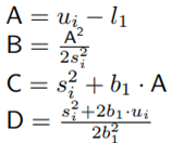
In order to improve the computational performance and the analytical treatment of the method proposed by Schwartz-Yeh, we need to find a function that approximates ξ (·) (Equation (17)] using a fewer number of terms. It also must be easily integrable. Therefore, the proposed solution in our work for ξ (·) is hereafter Equation (20) with the parameters: a n , b n , l n , where n only takes the value 1 or 2 to indicate the 1st and 2nd polynomial degree, respectively. Figure 2 shows the comparison between Equation (20) against Equation (17) which evidences such an approach.
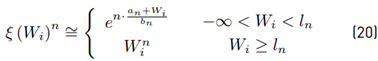
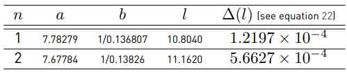
Parameters a n and b n were found through a nonlinear regression. The parameter ln is the closest intersection point of ξ (·) with the approximation given by Equation (20) (see Figure 2]. To find this point, we define l n as:
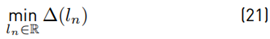
Where ∆(l n ) is given as a Riemann integral.
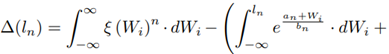
Table 1 Comparison of Monte Carlo simulations and analytical results using the Fenton-Wilkinson method. Expe=Experimental
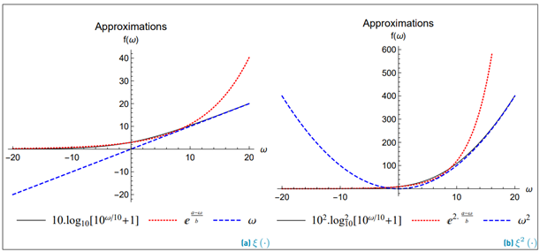
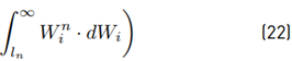
Equation (22) seeks to approximate the areas of both functions Equation (17) and Equation (20). The evaluation of the minimization has been done through numerical integration, and the exact parameters used with Equation (20) are listed in Table 2.
Next, we proceed to calculate the moments of the function ξ (·). We have for any i > 1 that:

Then:
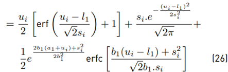
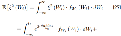
The first moment is:
And the second moment is:
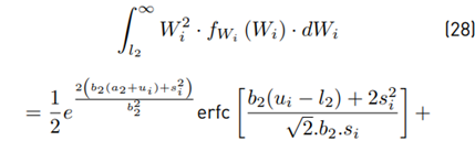
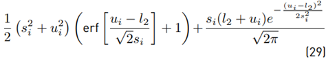
We can use Equations (26) and (29) to calculate the variance:

Hereinafter, we must calculate the mean value and variance in each i iteration as follows.
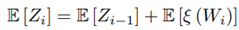
Calculating the mean value E [Z i ] We have Equation (19) as:
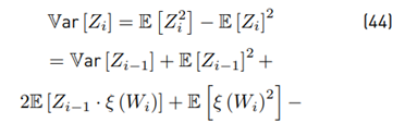
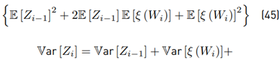
Calculating the variance Var [Z i ] Due to

because Wi and Zi−1 are correlated, we need to seek an alternative way to give a solution. Then, calculating first

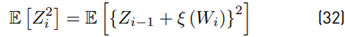

Then
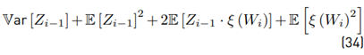
The term 2E [Zi−1 · ξ (Wi)] must be treated carefully because both variables are not independent. Based on [8], we have that:

Where:


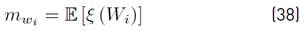
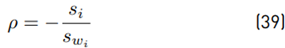
The term E [(Wi − m wi ) ξ (W i )] is calculated using our approximation proposed in Equation (20).
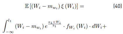
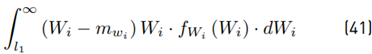
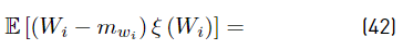
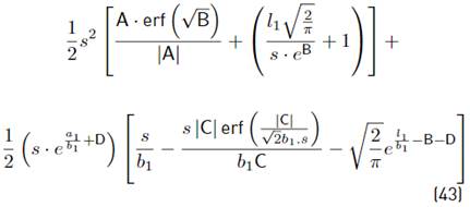
Where:
And finally, we have:

Now with E [ξ (Wi)] using Equation (26), Var [ξ (Wi)] using Equation (30) and 2E [Zi−1 · ξ (Wi)] using Equation (35), we have all equations to be used together with Equation (46), which can also be rewritten as:
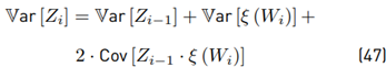
Where: Cov means covariance. Finally in this section, we have found all the formulations to evaluate E [ξ (Wi)], Var [ξ(Wi)], E [Zi], and Var [Zi] through the Equations (26), (30), (3), and (46), respectively.
4. Validation and analysis
We are going to validate our formulas by comparing them against the results of the Monte Carlo simulation. For this aim, we sum different numbers of RV’s with a wide range of parameters. The difference between the theoretical and experimental results are shown in Tables 3, 4, and 5. In this way, we can show that the approximation for ξ (·) let us calculate the mean value and variance for Z with a low error, even when the range of RVs are N = 20, and the parameters are m ∈ [−80, 80] and s ∈ [6, 12].
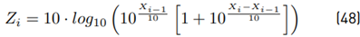
Explanation of Monte Carlo simulations 4,5 and 6 used to analyze Equations for E [Z] and Var [Z] We want to assess Equations 3 and 46 through simulations. Simulation number 4 analyzes the sum of only two lognormal RVs, N = 2. Then, we generate 107 samples for X i following a Normal PDF with parameters m i , s i and finally, we calculate Equation (49). From this result, we get the experimental mean value and variance. We repeat this procedure 4 times with different parameters mi and s i .
Simulation 5 and 6 follow the previous procedure, using N = 10 and N = 20 RVs, respectively.

The 3rd result in Table 4 and the 4th result in Table 5 show the maximum variance difference between the theoretical and the experimental. On the other hand, this method is based on the work of Schwartz-Yeh, but with a lower number of terms. To validate the performance of the method, two metrics are taken into account: error of the mean value and error of the variance.
The perceptual error of the mean value: It is the difference between the experimental (by means of Monte Carlo simulation) and the theoretical result. This error will be percentual using as a reference the experimental result. The way to calculate this value is:
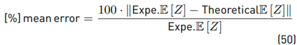
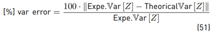
Percentual error of the variance: It is the difference between the experimental and the theoretical result of the variance. This error will be percentual using as a reference the experimental result, and the way to calculate this value is:
The proposed method has no restrictions with respect to m values and s values of each RV. However, the numerical evaluation must take into account the quantization error. That is why we must look for methods to reduce the error with respect to the analytical model proposed. Our initial approach was aimed at characterizing the sum of lognormal variables in a telecommunications scenario (where it is usual to take values for m = [−80, −60]); however, in our assessment, a greater range for the mean value was used m = [−80, 80].
When we evaluate 10 X10i , very small or large numerical values can be generated which leads to errors due to rounding. To reduce the rounding error, it is important that when we calculate Equation (15), the order of the variables is chosen in such a way as to guarantee that W i ≥ 0. Another important aspect is to analyze how the value of ˜µ, σ˜ changes in each iteration. The order of a set of N lognormal RVs does not affect the result of ˜µ, σ˜ analytically. But in the numerical evaluation, it is observed that for the same set of random variables, the result can change according to its order. The results of simulation 6 show that the error of the mean value is usually below 0.5 %, whereas that the error of σ˜ can change drastically from 20 to 0.1 % just with an adequate ordering of random variables. Through experimental processes, it was found that σ˜ is more sensitive to the values of mi instead of s i .
Explanation of simulation 7 used to determine the effect of ordering For different orderings, we are going to calculate the error metrics of our method using as a reference Monte Carlo simulation. In this case, we use 10 Normal RV’s X
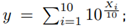
i
, i = {1, ..., 10} with parameters randomly selected for the mean value and standard deviation from m = [−80, 80] , s = [4, 20] respectively. For each RV 106 samples are generated. After that, the following operation is performed:
 and we calculate Y = 10 · log
10(y).
and we calculate Y = 10 · log
10(y).
Table 3 Assessment with N = 2, samples for each RV =106
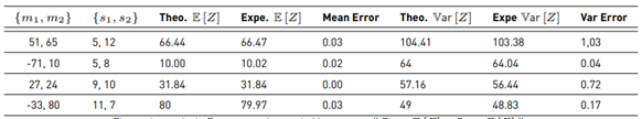
Theo.=theoretical, Expe.=experimental, Mean error=∥ Theo. E [Z] − Expe. E [Z] ∥, Var. error=∥ Theo. Var [Z] − Expe. Var [Z] ∥
Table 4 Assessments with N = 10, samples for each RV =106
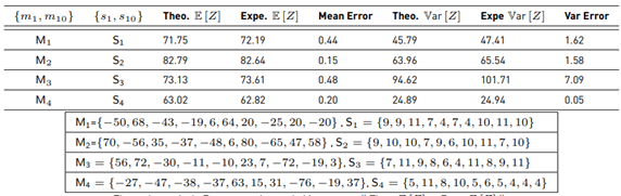
Theo.=theoretical, Expe.=experimental, Mean error=∥ Theo. E [Z] − Expe. E [Z] ∥, Var. error=∥ Theo. Var [Z] − Expe. Var [Z] ∥
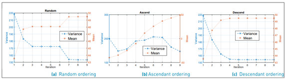
For each set of m and s, we sort lognormal RVs according to m in three different ways: random, ascendant and descendant. We calculate the theoretical mean value and variance of Y in each order, and these results are compared against the experimental results given by Monte Carlo.
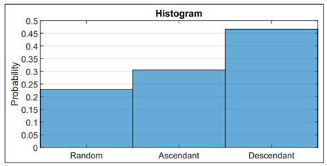
Finally, we choose the ordering with the smallest error. This procedure is done 106 times to know which ordering gives the smallest average error for the variance. To understand this phenomenon even better, as an example, we plot the evolution of µ˜ and σ˜2 in each iteration for each kind of ordering [Figure 3a-3c). The overall result is shown in Figure 4 as a histogram, where we can see that the smallest error occurs when the order is descending (with a probability of 47%). Note that the smaller error is reached with a descending order because the values converge asymptotically in each iteration. Meanwhile, in random and ascending ordering, abrupt changes of these metrics in each iteration are observed. (see Figure 3a-3c)
Table 5 Assessment with N = 20, samples for each RV =106
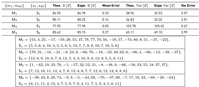
Theo.=theoretical, Expe.=experimental, Mean error=∥ Theo. E [Z] − Expe. E [Z] ∥, Var. error=∥ Theo. Var [Z] − Expe. Var [Z] ∥
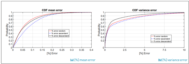
In order to give conclusions, we characterize statistically the behavior of the error metrics through their CDF. Figure 5 shows the CDF of the error for both metrics: the error of the mean value and the error of the variance for each ordering. It is noted that the error in the mean value µ˜ is below of 0.2% (with a probability of 90% of the time) in all orderings, while the error in σ˜ is below 3% (with a probability of 90% of the time) for descending order.
5. Conclusions
In this paper, we have proposed an efficient method based on the Schwartz-Yeh’s work for calculating the mean value and variance of the sum of lognormal variables. We use Equation (17) as a recursive process in conjunction with our Equations (3) and (46) to find the mean value and variance. When compared to other methods in the literature, the benefits of our method are: 1) Computational efficiency because Equation (17) was expanded in 40 terms in previous works, now we use only two terms. 2) Low error and useful in many fields because it can be used with a wide range of parameters. Take into account that the order of the terms of the sum does matter due to the numerical evaluation (the rounding errors). Therefore, we want to highlight that the best results are obtained when (a) the variables are processed in descending order with respect to their mean, and (b) W i ≥ 0 is guaranteed.
The validation of the proposed method has considered ranges for random variables with parameters m ∈ [−80, 80] and s ∈ [6, 12], and the descending ordering showed that the error for µ˜ is below 0.2% and the error for σ˜ is below 3%, both cases with a probability of 90% of the time.

