1. Introduction

In the traditional electricity distribution system, the electricity generated is taken to the end-users. In recent decades, distribution networks have been seen to have loads controller (LC) and distributed energy resources (DERs) in order to provide electricity service to small areas, thus increasing the reliability of the provision of electricity [¹-³].

A microgrid can incorporate renewable energy sources (RES) such as distributed generators (DGs) and battery energy storage systems (BESS) as a backup source in case it cannot generate power due to weather (for example, cloudy sky in the case of photovoltaic panels or low wind speed in the case of wind turbines) [⁴-⁷].

Voltage inverters in the RES are required due to their own characteristics in the power output. In addition, because inverters provide a quick power balance, it is necessary to implement a control scheme that will be key to the isolated operation of the microgrid [⁴,⁸,⁹] . This new grid configuration works as a support to the electrical system in case the main network is intermittent in the electricity service due to scheduled events or failures in the system [¹-³,⁷,¹⁰,¹¹]. By adding more DG units that have the ability to be automatically configured when connected to the microgrid.

The new configuration also provides challenges in isolated and connected modes, where cooperation between multiple DG units is key to providing the power corresponding to system demand in case the main network is unavailable [¹²-¹⁴].

Distributed control allows the system to accommodate an event by having the availability of local information, so when a failure occurs in any generation unit the distribution system does not shut down and does not generate a cascade failure. This is possible because the controller of each generating unit can communicate with the other controllers and strategies are established to maintain the power balance of the microgrids, reaching a consensus on the power they must generate [⁵,¹⁵,¹⁶].

Optimal control enables the operational constraints of the system to be met under all operating conditions, taking into account the uncertainty and variability associated with the output power of the RES, as well as the variability of the load.

A multi-objective scheme allows for the integration of multiple constraints subject to systematic physical and/or operational constraints, for example, minimising power consumption when the microgrid operates in isolation, power losses and associated operating costs [⁷,¹⁷-²¹].

Recently, alternative methods have been developed to achieve optimal globally distributed control [¹⁹]. In [²²], a simple real-time dynamic algorithm is proposed for energy management strategy. In [²³], presented a delay-free-based distributed algorithm to achieve the optimal economic dispatch. And in [²⁴], a distributed dynamic algorithm is used to solve an economic dispatch problem.

The consensus algorithm and an innovation term allows finding an algorithm that combines the cooperation between agents and the incorporation of their observations, where at each step of the algorithm the observations of the states of the neighbouring agents are processed [²⁵] .

In this paper, we present an optimal distributed control algorithm for a low voltage distribution system that includes microgrids as support systems and ensures the distribution of power between agents (DG, BESS and/or RES) and the demand for microgrids. The proposed approach is based on the consensus + innovations method [²⁵]. Although several studies have been carried out for the consensus control + innovation technique in microgrids [²⁶], the control of several AC microgrids connected to the distribution system has not been extensively studied and it is the main contribution of this work.

2. Preliminaries and notations

This section overviews the power flow equations, the Optimal Power Flow (OPF) formulation and Karush-Kuhn-Tucker conditions that are used in later sections.

2.1 Power flow representations

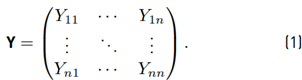
A power system of ^ith nodes is made up of n loads and m generators. Each node may be characterised by node-specific parameters such as generated power , demand power , node voltage and voltage angle [²⁷,²⁸]. To determine the control variables of the i node, it is necessary to model the power system using the admittance matrix Y (1), where each item on the matrix corresponds to the admittance values of each line and node. It is a n × n matrix with dimensions equal to the number of nodes and it is symmetrical along the diagonal and each item contains the electrical parameters of the node and the information of the network topology [²⁸]:

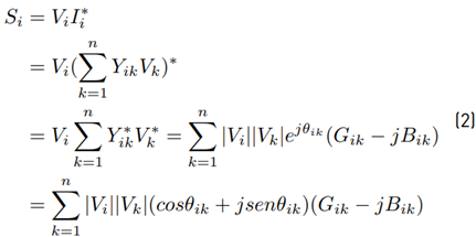
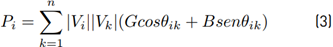
The net injected power given by Equation (2), at any node can be calculated using the node voltage V _i , the neighbouring node voltages V _k and the admittances between the node i and its neighbouring nodes Y _ik [²⁹,³⁰].

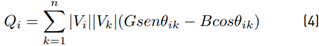
Thus the power flow in (3) and (4) Equations, at the i node is:

2.2 Power flow representations

An objective function to be optimised is defined, where voltage and frequency parameters are included, and corresponds to the cost function of the microgrid subject to linear and nonlinear constraints defined in the framework of the problem; thus ensuring stability by meeting the operational limits of the network and its economic efficiency [¹⁶,³¹].

The constraints limit the injection of power and voltage. In this way, the power flow in the network is maintained. Therefore, optimising the performance of the system according to a specific objective function is called an optimal power flow (OPF) problem. The general Equation (5) describes an OPF problem:

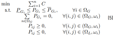
Where is the power of the generator are the maximum and minimum of power generation limits for the generator i ∈ N; P _ij is the power of the connected line among the nodes i and j; Ω _G and Ω _L are the sets of all generators and loads (or consumers) respectively; and ω _i is the set of all generators connected in the node i. The cost function C is usually based on generation costs, generation losses and the desired voltage; the function can be modeled by a quadratic function 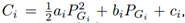Where a _i , b _i , c _i are the costparameters. [²⁹]

Solving the OPF problem results in the correct power flow in the network, keeping the values within the system constraints. With the appropriate control techniques, the ability to find an optimal solution globally is obtained, if the solution meets the conditions of optimality. The Lagrange method is used to remove inequality restrictions in variables. It turns the problem with equality restrictions into a problem of free optimal. Therefore, the function of Lagrange (6) is given by:

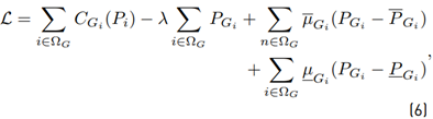
where λ, µ > 0 are the Lagrange multipliers.

2.3 Karush-Kuhn-Tucker conditions

Karush-Kuhn-Tucker (KKT) optimal problem conditions allow finding if the solution is optimal. Suppose a function f: K ⊂ ℜⁿ −→ ℜ is convex if K is a set of convex vectors and the constraint function is g : K ⊂ ℜⁿ −→ ℜ (7).

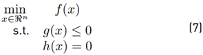
In this case, the optimal solution should be solutions of conditions (8):

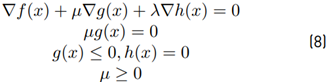
Therefore, assuming that f and g are continuously differentiable. If the pair (λ, µ) meets the KKT conditions described in Equation (8), x is an optimal solution to the problem. Additionally, if f is strictly convex, x is the only solution to the problem [³²].

3. Consensus+innovation: Decomposition-based control technique in a microgrid

The consensus + innovation technique is based on a multi-agent structure and where the agents in the microgrid coordinate their control parameters in a distributed way, ensuring the interoperability of the system and thereby allowing the ability to be plug-and-play [³³]. By not requiring a central agent, each agent defines its role on cost/demand and its constraints on local energy production and consumption, so that agents do not need to know the total demand for the system [²⁵].

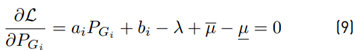
The C+I technique uses an iterative algorithm that allows all variables fluctuate in a subproblem and that at a limit point, the KKT conditions are satisfied, thus achieving a distributed solution of the KKT conditions[²⁹]. In the case of a convex problem, any limit point of the algorithm is an optimal solution [³⁴]. According to the first-order optimality conditions described in Equation (8), we obtain in Equation (6) the conditions presented in the Equations (9) - (12):

So to solve the previous system of first-order constrained equations in a distributed form, a distributed estimator is proposed, where each node exchanges information with its neighbours at each iteration and updates the variables associated with the node. The iteration counter is denoted by k and the iteration by X _i (k), which includes the variables associated with the i bus in the k iteration, for example X _i (k) = [λij (k), P _i (k)], thus the general form of the estimator distributed for each agent is defined by the Equation (13) [³⁵]:

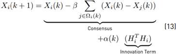
where (i, j) represent neighbouring agents to each other. Ωi denotes the communication neighbourhood of the agent i. α, β > 0 are the adjustment factors or consensus weights and innovation potential, respectively, and are defined by (14):

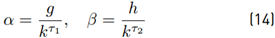
where g, h > 0, 0 < τ2 < τ1 < 1 and τ1 > τ2 + 1/2. Adjustment factors satisfy the following conditions:

1. The sequence of both factors sum to which is a standard requirement in stochastic approximation algorithms to drive updates to the desired limit of arbitrary initial conditions.

2. As the iterations increase, k → ∞, sequences of the parameters α and β decrease to zero, α → 0, β → 0.

3. The potential for asymptotic consensus dominates the potential for innovation, β/α → ∞ when k → ∞.

In addition, the square summation of α (τ1 > 1/2) is required to mitigate the effect of stochastic detection noise disrupting innovations.

The innovation term corresponds to the distributed observability of the system. The system observation is observable distributed if the matrix G is full rank (15) [³⁶]:

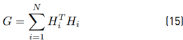
where G is the Gain matrix and consists of the Jacobian measurement H _i = [H ₁ , ..., HN ], associated with boundary measurements; and the covariance matrix of the measurement error R, in which it is assumed that on the diagonal has the measurement variations [²⁷,³⁵].

In this way, the consensus algorithm ensures the cooperation between the agents on the prices of the energy, and the innovation part allows the understanding of each agent on its observations, where the last part guarantees the fulfilment of the constrain Thus, combining these two algorithms is reasonable when each agent converges on an estimate of the N-dimensional field [²⁵,³⁶].

The Lagrange multiplier λ _ij is the estimated price vector of an agent i. The convergence of the price estimate is achieved in the update of Equation ⁽¹⁶⁾, through a consensus term corresponding to the conditions of optimality and evidences the coupling between the agent’s Lagrange multipliers. The second term constitutes a term of innovation and ensures the application of the restriction of equality:

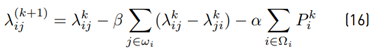
where α, β > 0 are the adjustment factors and k is number of iterations. ω _i is the communications neighbourhood of the agent i according to the network communication topology, Ω _i denote the set of generators of the grid. Settings of the parameters (α, β) are important for the performance of the algorithm and is usually a trade-off between convergence speed and configuration change resistance. The adjustment depends on both the value of the parameters and the relationship between the two. Performance could be improved by using adaptive factors that adjust this relationship.

The objective is to determine the generation dispatch in the microgrid to reduce the cost of supplying power to the demand, taking into account operational constraints such as generation capacity and limits in the distribution lines. If in Equation (9) for all system agents, the generated power P _Gi has not reached the upper or lower limit (µ̅ = 0, µ̲ = 0), then the optimal solution is for all agents to have the same marginal cost.

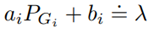
This is known as the economic dispatch criterion. For generators with binding inequality constraints the marginal cost is deviated from λ by the value of the Lagrange multipliers of the corresponding link constraints [³³].

Assuming that the primal problem supports a feasible solution, the optimal configuration for all agents can be parameterized only in terms of λ, thus knowing the value of the Lagrange multiplier λ _ij , the upgrade for the generator power i is given by (17):

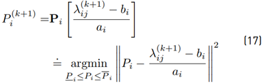
where Pi[·] denotes the projection operator associated with agent i, this operator projects the argument into the space of the feasible solution [P̲_i, P̅_i], where P̲ _i = max(P̲ _i , P_n,−1 + ∆P̲ _i ) and P i = min(P _Gi , P _n ,−1 + ∆P̅ _i), that is if the power values are greater than the upper limit (P̅ _i ) then the value of P _i ^(k+1) would be the upper limit and likewise for the lower limit.

Therefore, the maximum and minimum restrictions are adjusted to take into account the effective generation rate, where the initial output power of the generator is denoted by P _n ,−1. Under this approach, active power upgrade is equivalent to using Equation (9) where Lagrange multipliers µ̅ and µ̲ are included to upgrade the power. Additionally, it should be mentioned that as these multipliers do not appear in any other restrictions, it is not necessary to provide them with an update.

Thus, according to the equilibrium restriction of the power flow given in Equation (11), the objective of the distributed algorithm can be formalised as a restricted consensus problem, where agents seek to reach an agreement on the marginal cost λ.

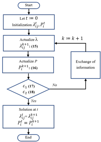
At each step of the algorithm iteration, only the local information is used from neighbouring agents, where each agent can represent a node or a region of the network and share the information of its variables (phase angle, generated active power and dual power balance variables) to the neighbours. Variables are used to calculate an update for the next iteration [²⁹].

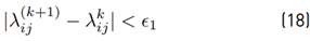
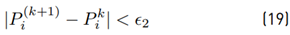
The flow diagram of the algorithm updates is shown in Figure 1, where the criterion for stopping the algorithm is when convergence is achieved, tolerance parameters are defined ϵ1 and ϵ2, where if the conditions (18) and (19) are met, the algorithm shall be terminated:

3.1 Convergence conditions

To ensure the convergence of the algorithm, the following conditions must be met:

1. Local innovation functions should be sufficiently regular.

2. The inter-agent communications network needs to be connected.

3. The adjustment factors (α, β) must satisfy the conditions described above.

In that sense, the sequence of weights or adjustment factors must be carefully designed, so the consensus of potential must master the innovation potential, to achieve convergence. The combination of two potentials makes the distributed algorithm and its convergence analysis fundamentally different from iterative approaches based on classical gradients.

Figure 1 Flowchart of the Consensus + Innovation algorithm updates 

4. Simulations

The test system in Figure 2 is derived from an IEEE 34 nodes test feeder, the DGs are located at nodes 848, 840, 828, 806 and 824, the BESS is placed at the node 890.

Figure 2 Test system based on the IEEE 34 nodes test feeder with microgrids 

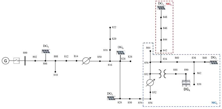
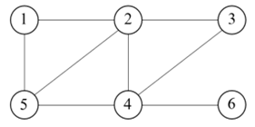
We can observe Microgrid 1 and Microgrid 2 on the test feeder. The network connects to the main grid at node 800. PV generators are considered to have the same characteristics. The communication connections between the DGs are shown in Figure 3, each agent corresponds to a system DG and the graph adopts a different topology to the physical connections of the system.

Figure 3 Communications topology between agents 

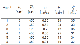
The parameters for PV generators and battery are shown in Table 1. For system simulations, initial values are taken from the Lagrange multiplier λ, corresponding to the energy price in each DG. It is assumed that the minimum active generation power for DGs is 0kW, thus the variable P is initialised at zero. Additional, in order that generators will be indispensable, it is defined that the difference between maximum and minimum limits is equal, that is ∆P̲i = ∆P̅i, allowing to define a virtual cost function a _n and bn without affecting the optimal solution.

Since the convergence speed of the C+I algorithm depends on the adjustment parameters, after several combinations the following parameters are chosen (20):

Table 1 Parameters of the system generators 

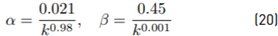
Where k = 1, ..., N is the iteration counter. The tolerance parameters defined in Equations (18) and (19) are defined as:

In order to evaluate the performance of the algorithm in isolated state and connected-mode to the network, in the first simulation, an isolated system is taken from t = 0s to t = 0.4s, from t = 0.4s to t = 1s the system is connected to the main distribution network and from t = 1s the system disconnected again to the main distribution network.

Figures 4 and 5 show the behaviour of the marginal cost, λ, of each agent. It is observed that the marginal cost of each agent tends to stabilise prior to the disconnection of the system to the main network. In the first time interval t = (0; 0.4]s, all the agents keep the initial price. For the interval t = (0.4; 1]s, all the agents decreased their costs since the system connected to the main distribution network. In the last interval of time t = (1; 2]s all the agents reached the initial cost values.

For this first case, in the time interval t = (0.4; 1]s all the agents decreased the cost of generation, agents 1 and 2 decreased in 30.18% and 32.91%, respectively. The agent 3 decreased in 7.24% the cost of generation, it can be observed that in t = 1s the value reaches a minimum cost of 19.47 $/kWh. Agents 4 and 6 decreased the cost in 51.93% and 54.35%. Agent 5 reaches a minimum cost of 2.37 $/kWh at t = 0.99s.

At t = 2s it can be seen that agents 1 and 2 converge at 34.09 $/kWh and 33.35 $/kWh, respectively. Agents 3 and 4 converge to 33.53 $/kWh and 32.46 $/kWh, respectively. Finally, agents 5 and 6 reached the initial cost values, 32.17 $/kWh and 33.21 $/kWh.

From the results obtained for marginal costs present in Figures 4 and 5, it can be inferred that thanks to the adjustment parameters α and β a rapid convergence is obtained for each agent, it can be seen that before starting each interval, the cost converges to a value.

Figure 4 Evolution of the marginal cost λ of agents 1, 2 and 3, located at nodes 1, 2 and 3 

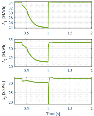
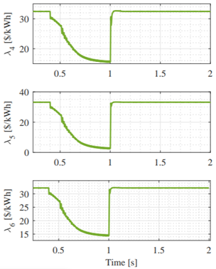
Figure 5 Evolution of the marginal cost λ of agents 4, 5 and 6, located at node 6, 8 and 10, respectively 

Also, it is observed that in the connected mode, there is a variation in the cost and it converges before starting the next time interval.

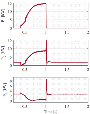
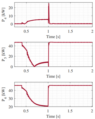
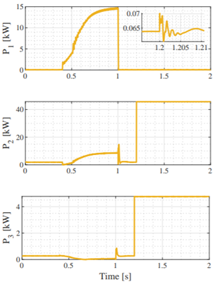
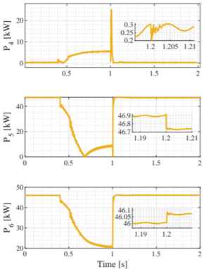
Figures 6 and 7 show the evolution of the active power of each of the agents. It can be seen that the power in each agent converges to a specific value in each time interval.

It is observed that the convergence is achieved at a value in each agent, in the first interval t = (0; 0.4]s the agents keep the initial power. In t = (0.4; 1]s the agents 1, 2 and 4 increased the power generation in order to balance the power generation in the connected mode, increasing the generation until 14.59kW for the agent 1, 8.71kW for the agent 2, and 5.44kW for the agent 4. Agents 3, 5 and 6, on the contrary, they reduced their power generation by 78.79%, 78.73% and 55.61%, respectively.

In the third time interval t = (1, 2]s, the generating power returns to the convergence values of the first time interval. Additionally, it is noted that the power for each agent depends heavily on the values of ai and bi and the minimum and maximum limit power restriction in the generator allows each generator to be within the desired generation interval.

At t = 2s, the active power of agent 1 reaches 0.062kW of generation; agent 2 reaches 1.823kW; agent 3 generates

Figure 6 Active power of the agents 1, 2 and 3 

Figure 7 Active power of the agents 4, 5 and 6 

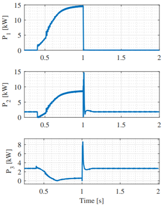
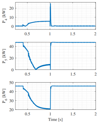
2.757kW, agent 4 reaches 0.3155kW; agent 5 has the highest generation of active power with 46.91kW and finally, for agent 6 reaches 46.02kW. This shows that the active power depends directly on the marginal generation costs obtained in the update of the parameter λ and also depends on the values given for the parameters a _i and b _i .

4.1 Loss of physical connection

To check the convergence of the technique, the line loss between nodes 842 and 844 is simulated at t = 1.2s. The loss of the line between the two nodes would leave two (2) microgrids (MG₁ and MG₂) without physical connection, reconfiguring the topology of the system.

Figures 8 and 9 show the marginal cost of each DG when a line is lost from the network either by failure or opening for maintenance.

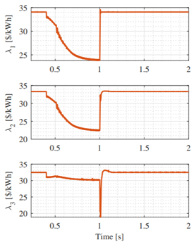
Figure 8 Evolution of the marginal cost λ of agents 1, 2 and 3 when there is a loss of the line between buses 5 and 6 

Similar to the above analysis, the system is isolated in an initial mode at the time interval t = (0.4; 1]s. The cost behaviour evolves in a way comparable to the previous result. The communications layer allows agents to exchange information between neighbours obtaining convergence in individual costs. It can be seen that similar to the previous case, all the agents decreased the cost of generation in the time interval t = (0.4; 1]s, and even in almost the same percentage of change for all agents as the previous case. It can be seen that the disconnection of MG₁ at t = 1.2s does not affect the convergence of the individual costs for the agents.

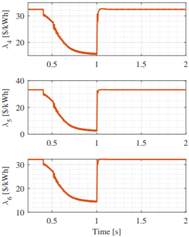
Figure 9 Evolution of the marginal cost λ of agents 4, 5 and 6 when there is a loss of the line between buses 5 and 6 

The behaviour of the active power of each generator is observed in Figures 10 and 11. Similar to the analysis in the previous section, the active power depends on the marginal generation costs, λ, and the values given for the parameters a _i and b _i . Additionally, it can be seen the same behaviour as the previous case.

At t = (0.4; 1]s, agents 1, 2 and 4 increased the power generation until 14.34kW, 8,39kW and 5.65kW, respectively. Agents 3, 5 and 6 decreased the power generation by 79.53%, 83.35% and 55.41%, respectively.

At t = (1; 2]s, as the first case, the generating power returns to the convergence values of the first time interval. The results show that through the communication connections among the different agents, there is a reconfiguration in the generation. Obtaining as a result increases or reductions in the power generation of all agents. In comparison with the previous case shown in the Figures 6 and 7, the active power for agent 5 in the last time interval show a decrease in 21.7% with respect to the power value of the first case.

Figure 10 Active power of agents 1, 2 and 3 when a line between two nodes is lost 

Figure 11 Active power of agents 4, 5 and 6 when a line between two nodes is lost 

4.2 Loss of communication links

In this case, the system loses a communication link between agents 2 and 3 at t = 1.2s, thus configuring the communication topology of the system. For this new communications network agent 3 lose the exchange of information with agent 2, so its only means of collecting information from the system is the connection with agent 4.

Figures 12 and 13 show the marginal cost of each DG when a communication link is lost. In this case, the communications layer is affected by the loss of a link, as seen in the figures, the cost of each agent has minor variations after the communication disconnection.

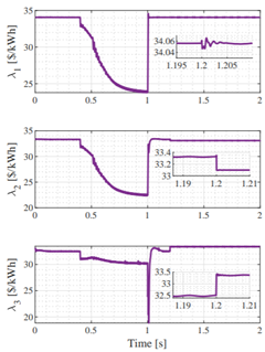
Figure 12 Evolution of the marginal cost λ of agents 1, 2 and 3 when there is a loss of the communication link between agents 2 and 3 

Agents 1 and 5 converge to the same cost before t = 1.2s. Agent 2 decreases their cost by 0.66% with a final cost of 33.1 $/kWh. Agent 3 increases the cost by 2.65%respect the cost at t = 1.19s, reaching a final value of 33.37 $/kWh. Finally, agent 4 increases in 0.34%the cost of generation taking into account that the only communication link for agent 3 to the system is through agent 4. It can be seen that the value of λ increases or decreases depending on the new communication topology.

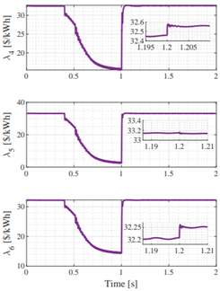
Figure 13 Evolution of the marginal cost λ of agents 4, 5 and 6 when there is a loss of the communication link between agents 2 and 3 

It is evident that in agent 3 the cost of generation increases when it is disconnected from much of the network and remains connected to the system through only a communication link with agent 4.

Figures 14 and 15 show the behaviour of the active power of each generator when a communication link is lost, in this case between agents 2 and 3.

Similar to the results of Figures 4 and 5, the behaviour of the power generation in all agents before t = 1.2s is similar at the previous study cases. At t = 1.2s, agents 1 and 5 has a minor variation the power generation, decreasing by 1.39% and 0.34% the values respect the time interval t = (1; 1.2]s.

It can be observed, agent 2 has the highest rate of increase in generation, reaching a final value of generation of 45.69kW. Agent 3 reached its maximum generation value of 4.76kW. Finally, agents 4 and 6 have minor variations in the generation increases in 0.20% and 0.13%the cost of generation, respectively. The figures show that the variances are due to the disconnection of the communications link between agents 2 and 3.

Figure 14 Active power of agents 1, 2 and 3 when a communication link is lost 

Figure 15 Active power of agents 4, 5 and 6 when a communication link is lost 

4.3 Replicator dynamics algorithm

In this section, the results of the distributed dynamic dispatch algorithm proposed in [²⁴], depicted in Figure 16.

It is observed, when the system is connected to the main grid at t = (0.4; 1]s all agents increase the power dispatch, increasing the generation 7.85% for agent 1, 3.43% for agent 2, 22.48% for agent 3, 16.23% for agent 4, 26.39%for agent 5 and the highest increase in agent 6 with 27.89%.

Figure 16 Dispatched power and frequency response of all six DGs 

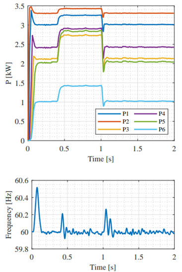
It can be inferred from these results that, as in the Figures 6 and 7, the agents increasing their generation in order to balance the power generation in the connected mode.

The frequency response shows that the system keeps the frequency stability in the isolated mode.

5. Conclusions and future work

The consensus + innovation control technique has striking advantages for OPF problem solving in distributed systems. The variable update directly makes a computational and practical advantage to obtain an optimal distributed solution in solving the power flow distribution problem. The operational constraints of the system are contemplated in the design of the controller, it is formulated as an OPF problem in which the aim is to minimise the generation costs of each agent subject to the constraints imposed by the system and its capacity. The Lagrange method makes it easy to see the problem as a problem of free optimal, such compliance with the KKT conditions allows finding the optimal points of the OPF problem. In this way, the update in each step of the parameter λ and the active power in each agent, allows finding the limit points of the algorithm and with it an optimal distributed solution for the system is established.

The convergence of the marginal cost of generation λ and the active power of each agent is evident in each case of testing. The communications topology allows to establish a network of information exchange between neighbouring agents, demonstrating the ability of the controller to respond to an eventuality in the physical layer of the system. The loss of a link in the communications layer demonstrates the controller’s ability to resolve the system’s OPF problem, even if the information from neighbouring agents is reduced.

The optimal distributed controller designed under the consensus + innovation technique allows the distribution of power flow throughout the system with communication links between neighbouring agents, thus achieving convergence between the state of the system without the need to have a complete communication network. In addition, the mere exchange of information on marginal generation costs between neighbouring actors reduces the information saturation in the communication links. Finally, the technique allows a fully distributed coordination in the components of the system.

Including considerations in distributed alternative techniques will greatly guarantee an improvement in the performance of the controller and allow a faster response, allowing them to have a lighter and more affordable computational performance. Communication with buses beyond immediate neighbours will enhance the convergence rates. Considerations of asynchronous updates could reduce the overhead in the communication connections of the system. Incorporate security constraints in the algorithm would enable the system to be secured against threats and protect end-users. Finally, including in the control technique more technical restrictions will improve the response on the system.