


 English (pdf)
 Article in xml format
 Article references
 Send this article by e-mail
 Cited by SciELO
  Cited by Google
  Similars in
SciELO
Similars in
SciELO  Similars in Google
 Permalink
1. Introduction
The operation and maintenance activities in photovoltaic (PV) plants can benefit from an accurate model of the expected PV plant’s power or current efficiency. PV operators can identify underperformance due to failures or soiling with this efficiency model, proposing new techniques such as [1-3]. Even though a PV module datasheet provides information that can be used to get an idea of the electrical characteristics of a PV plant, that information has been obtained under laboratory conditions which, in several cases, are different from outdoor conditions. Hence, measured experimental efficiency differs considerably from the efficiency reported in the PV panel datasheet, as has been verified in [4]. The difference above is not suitable for a PV plant’s proper maintenance and operation. Several PV efficiency models have been developed, i.e., Fifty-three models are presented in [5] and twenty-three are presented in [6]. Also in [7], an extensive study on empirical models is presented, which presents the errors comparison among 15 models. Several models are based on the model presented in [8] that defines the efficiency as a function of the temperature of the cell and the irradiance. Other types of models also incorporate the air mass (AM), such as the one proposed in [9]. Empirical models such as the one proposed in [10], or the one proposed in [11] have been accurate. But, the main disadvantage of the models mentioned above is that they require data sets and fitting algorithms to find optimal parameters. On the other hand, the efficiency models based on physical parameters, such as the one proposed in [12], have demonstrated a high accuracy with the IEC 61853 data. Still, also it requires a complex procedure to obtain the five fitting parameters.
It would be more appropriate to obtain an efficiency model that is accurate for outdoor conditions and calculated from reference points without any type of regression. In this regard, the present paper proposes an outdoor efficiency model that can be constructed with the standard data provided by the PV module datasheet or other efficiency points provided by norms, i.e., IEC 61853-1.
The proposed model is inspired by the fact that PV efficiency values plotted in a temperature, irradiance, and efficiency space resemble a surface when low irradiance values are not considered. In this regard, we demonstrate in this paper that it is possible to obtain a best-fit plane equation (BFPE) that estimates the efficiency of a PV module using irradiance and temperature measurements with reasonable accuracy. In addition, this paper also derives a simpler efficiency plane equation (PE) that can be obtained using the datasheet values of the PV module and that does not require the use of best-fitting techniques.
This article used several data sets obtained with different methodologies. The reference efficiencies obtained according to the IEC 61853-1 and the outdoor efficiencies were obtained by the National Renewable Energy Laboratory (NREL), which carried out all the data acquisition. In summary, we prove that a proposed PE model calculated from the power matrix is equivalent to the BFPE model calculated from a data set gathered during a whole year for several locations.
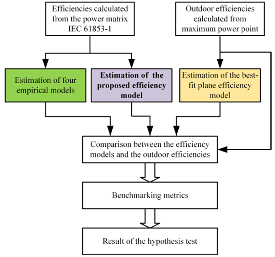
The methodology followed can be summarized in the following steps: First, we calculate the BFPE model from outdoor efficiency measurements. We selected six locations and a panel technology; then, we filtered the efficiency records in specific ranges of temperature and irradiance. The second step was to calculate our plane model, which was calculated from an efficiency dataset obtained from the power matrix according to the IEC 61853-1. Then, four models were used to compare their estimations with the proposed model. We used Evans’ model, Ransome’s model, Heydenreich’s model, and Durish’s model because they are widely referenced, as indicated above. The fourth step consisted of studying the fitting of the models and then hypothesizing about the similarities between the PE and BFPE models. The process mentioned above is summarized in Figure 1. The authors believe that the simplicity of the proposed PE model, along with obtained accuracy, makes this model an appropriate tool for fault detection and PV power production estimation when there are no historical efficiency measures available.
This work is an extension of the research presented at the Ibero-American Congress of Smart Cities (ICSC-CITIES 2021) [13], to which three new efficiency models were added to contrast with the data and our model. The use of more models changed the original structure of the work, adding, for example, new sections, new graphics, updating tables, etc. The rest of the document is structured as follows: section 2 presents a short review of the efficiency models and the proposed model, and section 3 explains the metrics used in the analysis, section 4 describes the experimental data analysis, and section 5 explains how the coefficients of the efficiency models were calculated. Section 6 explains the methodology for testing whether the proposed plane cuts the efficiency point cloud, and the analysis and result are presented in section 7. Finally, the main conclusions of this work are presented in section 8.
2. Efficiency models for PV modules
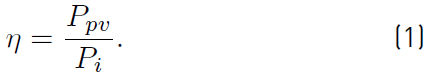
The efficiency of a PV module is the ratio between the output electrical power, P pv , and the received solar irradiance on its surface, P i , as indicated in Equation (1).
The input power is P i = Gi A, where G i is the sum of direct, diffuse, and ground-reflected irradiance incident upon an inclined surface parallel to the plane of the PV module and A is the area of the PV module.
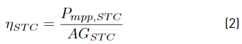
PV module datasheet provides rated efficiency values at given conditions, being the most common the efficiency at standard test conditions (STC),
 , as indicated in (2), where the considered output power,
 , is the maximum power that the PV module can produce at a temperature in the PV module of T
STC
=25 ◦C (298.15 ◦K), and incident irradiance of GSTC = 1000 W/m2 and an air mass of 1.5.
, is the maximum power that the PV module can produce at a temperature in the PV module of T
STC
=25 ◦C (298.15 ◦K), and incident irradiance of GSTC = 1000 W/m2 and an air mass of 1.5.
The STC efficiency of a 72-cell crystalline PV module ranges from 18 % to 22.8 % [14]. The efficiency of a PV module is not a constant value but depends on several variables and parameters, as shown next.
To illustrate the PV module efficiency dependence on environmental variables consider the ideal three-parameter model for a PV model shown in Equation (3), i.e.,
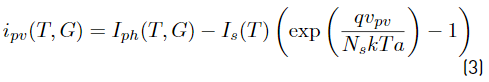
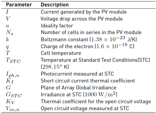
where the photocurrent I ph is defined according to (4), and the diode saturation current I s is defined according to (5). The variables and parameters used are defined in Table 1. According to [15] and [16], the influence of the temperature (T) and irradiance (G) in (3) can be expressed as,
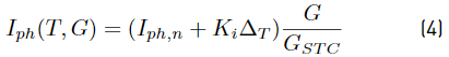
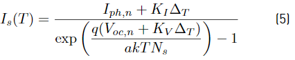
Table 1 Parameters used in the PV model. Standard Test Conditions (STC): Irradiance of 1000W/m2, a temperatura 298.15◦ K and an air mass of 1.5
where Δ T = T − T STC . Based on (2) and (3), it is possible to infer that the efficiency varies concerning the temperature. Even though the input power, P i , of the efficiency expression (1) does not vary with T, according to the simplified model shown in (3), the PV-generated power changes with respect to T. The aforementioned reasoning explains several efficiency models based on physics, such as [12,17].
2.1 Empirical models of efficiency
The empirical efficiency models define a function in terms of the PV module temperature, T, and the in-plane irradiance, G, i.e., η = f(T,G). In this regard, several authors (e.g, [18] and [6]) have proposed temperature-dependent efficiency models most of them derived from the seminal models presented in [8,17], where, in all cases, as the temperature in the PV module increases, the efficiency decreases reaching zero value at 270 ºC as indicated in [5]. It is important to highlight that the STC efficiency is an optimistic value given that a PV module temperature of 25 ºC occurs at low ambient air temperature. The Evans’ model (6) defines an expression for the efficiency as follows,

where η and η STC are the estimated efficiency and the efficiency at Standard Test Conditions (STC), and β and ζ are the temperature and irradiance coefficients, respectively. It is suggested that constant values for silicon panels of β = 0.0048 and ζ = 0.12 [8], but [6] shows that there might be a large variation in both parameters, i.e., β usually varies between [0.0026, 0.0060] depending on the technology of the PV cell/module.
As mentioned previously, the efficiency reported in a PV module datasheet is obtained from measurements with a constant air mass (AM) of 1.5. In photovoltaics, AM is used to approximate the effects of spectral responsivity in PV modules. Nevertheless, air mass changes according to the relative position of the sun and the molecules present in the atmosphere. According to [19], there is a 2% difference between the efficiency measured at AM 1.5 and AM 0. These other effects that take place in the PV module affect efficiency and they have been studied by some authors. For instance, the Durisch’s model [9] shows the efficiency expression as a function of the in-plane irradiance, PV module temperature, and air mass. Nevertheless, it is not uncommon that the majority of the PV efficiency models neglect the Air Mass; doing so for Durish’s model (7) yields the following simplified expression,
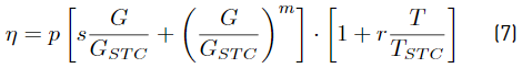
where T STC and G STC are the temperature and the irradiance at STC, respectively. The authors establish that the parameters p, r, s and m have to be identified for each type of solar cell/module. Another empirical model used in this work is the Heydenreich’s model [10]; the efficiency model (8), is expressed as,
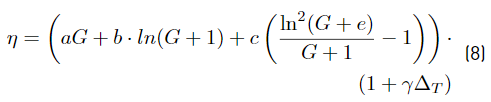
where {a, b, c} are the fitting parameters, and
 is the temperature coefficient at the maximum power point.
Ransome’s model [11] is normally called Mechanistic Performance Model (MPM), which is formed by six parameters. Still, we could neglect the parameter associated with the wind speed and the constant related to the inverse of the irradiance. In this way, the simplified expression (9) is the following,

where {c1, c2, c3, c4} are the constants linked to the efficiency, temperature and irradiance.
2.2 Proposed efficiency model
The simplest expression for the PV module efficiency η =f(T,G) is a linear function (10), i.e.,

where K1, K2 and K3 are constants. The parameters K1, K2 andK3 can be obtained from at least three points from the efficiency space, i.e., each efficiency point is defined by three values which are η, T andG. Assume that such three points are named as: P = ⟨Tp,Gp, ηp⟩, Q = ⟨Tq,Gq, ηq⟩ and R = ⟨Tr,Gr, ηr⟩, then an efficiency expression can be derived from the following set of equations,
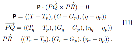
The solution of Equations (11) is obtained by solving the following determinant
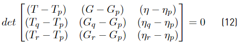
however, choosing special points where Tr = Tp and Gq =Gp allow us to solve Equation (12) easier. Then, comparing (10) with (12), it can be seen that parameters Ki are equal to (13),
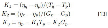
The constants K1, K2, and K3 can also be obtained from a set of experimental points using multivariate nonlinear regression techniques yielding a best-fit plane efficiency (BFPE) model.
In [20], the efficiency expression (10) was derived from values readily available in PV modules datasheets. By employing simulations, the authors were able to verify that the efficiency values obtained from the proposed model at different temperatures and irradiances had at most 2.6% difference with respect to more complex and validated models such as the Evans efficiency model, e.g. [8]. Nevertheless, in [20], no experimental analysis or validation was provided.
3. Metrics to compare the efficiency estimations
The metrics to evaluate the accuracy and precision of the models are based on the analysis of the residues. We consider the residue r
i
as the difference between the i
th
value of observed efficiency (ηi) and the estimated result by the model
 for the outdoor conditions (T
i
,G
i
) as follows,
for the outdoor conditions (T
i
,G
i
) as follows,
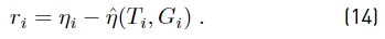
Notice that from (14), it is possible to obtain a relative error (15), i.e.,
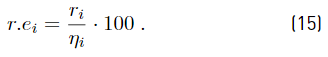
This metric explains how far the efficiency point is, predicted by the model from the point of view of the experimental data. Another metric used to compare the models is the normalized root mean square deviation (nRMSD) which is the RMSD value divided by a nominal value [21], and nRMSD (16) is defined as,
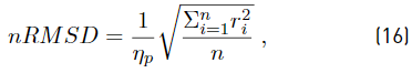
where n represents the number of elements to analyze.
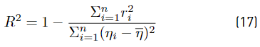
Also, the coefficient of determination, R 2(17), is used to determine if the variability of the data is captured by the model [22], and it is calculated as follows,
where
 is the average of the observed efficiency values ηi. The adjusted R2 (
 ) is shown in (18) and it is obtained as in [23],
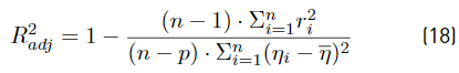
where p is the number of coefficients in the estimation model. Also, the mean of the relative error,
 (19), a type of percentage bias is calculated as,
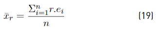
and the standard deviation of the relative error, σ r (20), which is calculated as follows,
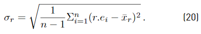
It should be noticed that the value of
 indicates on average how far the data are from the estimations of the selected model, and this value can be associated with the accuracy of the models. The other metric, the value σ
r
represents the dispersion of the relative error, and it can be related to the precision.
indicates on average how far the data are from the estimations of the selected model, and this value can be associated with the accuracy of the models. The other metric, the value σ
r
represents the dispersion of the relative error, and it can be related to the precision.
4. Experimental data used for validation
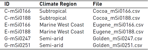
The data set used for validation was obtained from measurements made on four multi-crystalline PV modules, all of them having a surface of 0.3429 m2 and consisting of 36 cells connected in series. The data above was facilitated by the NREL[24] in the US, and it was taken in three different locations with distinct climates.
as indicated in Table 2. The data used for validation was taken with high-precision equipment as detailed in [24], and the measured variables were: plane-of-array (POA) irradiance with an uncertainty of 2.42% , the PV module back-surface temperature with an uncertainty of 1.76%, and the maximum power produced (MPP) with an uncertainty of 0.41%. This means that outdoor efficiency data have an uncertainty of around 3.02%.
The outdoor data used in this analysis were limited to PV module back-surface temperatures greater than 298.125 ◦K and less than 338.125 ◦K, a POA irradiance greater than 200 W/m2 but less or equal to 1050 W/m2, and a PV module soiling derate equal to one (clean panels). The cloud of points comprising the aforementioned range can be seen in Figure 2 for the case of a PV panel in Cocoa, Florida.
Table 2 Identification (ID) of the PV modules and the climate region from which the experimental data were obtained
With the measurements of temperature and POA irradiance, an experimental efficiency (η) has been calculated for each data point according to (1). In this way, a point located in a three-dimensional space (T, G, η) has been obtained for each PV panel and each geographical location. For instance, these efficiency values for module C-mSi0166 are shown as light-brown circles in Figure 3.
The NREL database also includes for every panel its power matrix following the IEC 61853-1: Irradiance and Temperature Performance Measurements and Power Rating [25], which describes requirements for evaluating PV module performance in terms of power rating over a range of irradiances and temperatures. These data are represented as blue asterisks in Figure 3, and later we used them as a reference to calculate the plain equation (PE) (10), and the four empirical efficiency model: Evans’ model (6), Durish’s model (7), Heydenreich’s model (8), and MPM (9).
5. Efficiency models
5.1 Proposed plane equation
The efficiency surface expression (10) is constructed using the following three points in the efficiency space:
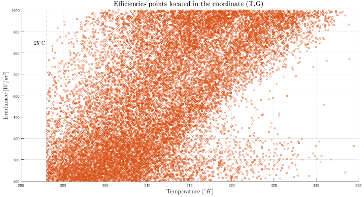
Figure 2 Data cloud considered for the validation of the efficiency expression. Case of module ID C-mSi0166 in Cocoa Florida
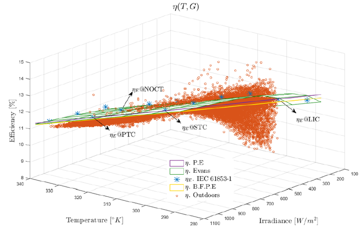
Figure 3 Efficiency values obtained at outdoors conditions (light-brown circles) and with IEC 61853-1 procedure (blue asterisks) for the PV module C − mSi0166. The presented efficiency models are: Evans efficiency expression (green surface), the proposed plane expression calculated from three reference points (purple line) and the best-fit plane model (yellow line) calculated from the outdoor efficiency measures
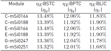
The point P is the equivalent efficiency obtained at the Standard Test Conditions (STC) point. This efficiency data point, ηE @STC, has an incident irradiance of G STC =000W/m2 and a back panel temperatura of T STC =25 ◦ C.
The point Q is the efficiency obtained at the high-temperature condition point and for this model, we selected the efficiency obtained at the PV-USA Test Condition (PTC) equivalent point. This efficiency data point, ηE @PTC, has an incident irradiance of G PTC = 1000W/m2 and a back panel temperatura of T PTC = 50 ◦ C. This point has been selected
due to the possibility of pairing it with the PV-USA Test Condition (PTC) point reported in some PV manufacturer data sheets, which is a US-standard that was developed in collaboration with the U.S Department of Energy [26].
The point R is the equivalent efficiency obtained at the Low Irradiance Condition (LIC) point. This efficiency data point, ηE @LIC, has an incident irradiance of G LIC = 200W/m2 and a back panel temperature of T LIC =25 ◦ C.
These reference points are calculated from the matrix powers given by IEC 61853-1 in the NREL database. Table 3 shows the experimental efficiency values obtained for the aforementioned three points for the panels under study.
Table 3 Experimental efficiency measures ηE calculated with the IEC 61853-1 for the standard conditions
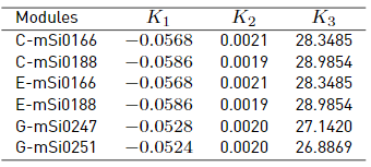
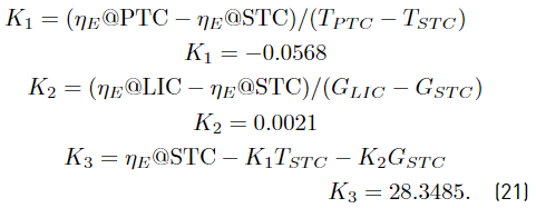
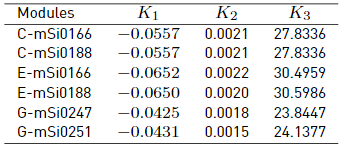
Using the efficiency measures in Table 3 and the expressions in (13), the constants of the Table 4 are obtained. The following example shows the calculus (21) for module C-mSi0166,
5.2 Empirical models of efficiency
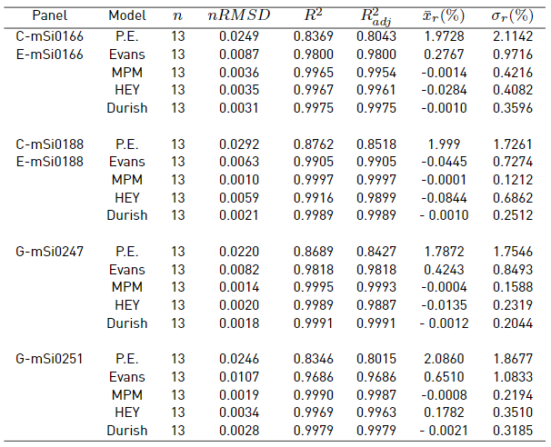
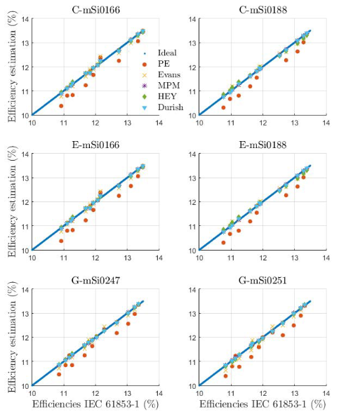
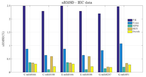
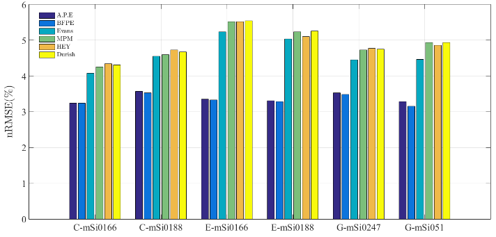
Following the procedure presented in Figure1, we adjusted four empirical models to the efficiencies calculated with the power standard IEC 61853-1. In total, six panels and four empirical models were adjusted. The fitting algorithm used was the nonlinear least-squares with a trust region(NLS-TR) of the Matlab Curve Fitting Toolbox [27]. Figure 4 shows the efficiencies derived from the IEC standard versus the efficiency estimation for all six panels. The diagonal blue line represents the perfect estimation, and data in the lower triangle means the sub-estimation of the models. On the other hand, data in the top triangle mean overestimation of the models. It can be observed that models with four parameters, such as MPM, HEY, and Durish, fit better than models with fewer parameters, such as Evans, with one fitting parameter. The goodness of the fit defined by Equations (16) to (20) for all the efficiency models and PV modules is presented in Table 5. Notice in general that the MPM model is the one with the best fit to the IEC data; for example, the normalized RMSD is lessthan0.4%, this metric is shown in Figure 5.
5.3 Best Fit Plane Equation
The best-fit plane efficiency (BFPE) model is obtained by fitting the constants{K1, K2, K3}to the outdoor efficiency data. This procedure was done with using the nonlinear least-squares with a trust-region (NLS-TR)algorithm of the same toolbox [27]. The results are shown in Table 6.
5.4 Visualization of the data: example
As an illustrative example of the data and some models, Figure 3 shows the aforementioned representations for the module C-mSi0166. In that figure, the outdoor efficiency values are presented as light-brown circles; the experimental efficiency values obtained with the power matrix according to IEC 61853-1 are presented as blue asterisks; the surface that estimates the efficiency using the model (10), with the three reference points, is the purple mesh and here it looks like a line. The BFPE model that estimates the efficiency using (10), with the parameters obtained from the data cloud (light-brown circles), is presented as a yellow mesh. Finally, the Evans’ efficiency model adjusted to the efficiency values obtained according to IEC 61853-1 (blue asterisks) is presented as a green mesh. In Figure 3, only the Evans’ model was presented to keep the readability of the figure.
The MPM, HEY, and Durish models are closer to the asterisk data. Therefore, these good fits, in some cases, hide the asterisks, and the models cannot be distinguished.
6. Validation methodology
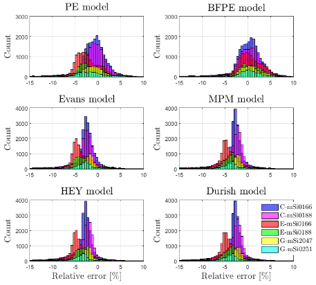
In order to prove that the plane equation behaves as well as the best-fit plane equation, the following steps have beendeveloped:1. For every PV panel, comparing the efficiency models estimated with the IEC 61853-1 data and, the outdoordata.2. For every data set selected, proving using the hypothesis test if the efficiency plane models could have equivalent precision and if they could have equivalent accuracy.Table7 shows the metrics calculated for the six efficiency model: the proposed plane efficiency (PE) model, the best-fit plane efficiency (BFPE) model, the Evans’ models, the Mechanistic Performace Model (MPM), the Heydenreich model (HEY), and the Durish’s model. The graphical distribution of the relative errors for all the efficiency models and PV modules is presented in Figure 6. Each subfigure is associated with a specific efficiency model, and inside there are six histograms related to each PV module. The mean and the standard deviation of these error distributions are equivalent to the ones calculated with Equations (19), (20), and are presented in Table 7.
6.1 Establishment of the hypothesis test
To quantify the similarity between the BFPE model and the PE model, 12 hypothesis tests are made with the data provided. The Minitab Software [28] was used to process the data. The hypothesis tests, formulated in Equation (22) were analyzed with the Bonetts’ method, and according to [28], this method is more rigorous than the Fisher or Levene methods. Another benefit is that Bonetts’ method can be used with data that do not have a normal distribution, therefore the normality test is not required. The hypothesis test proves if the standard deviation of the relative errors of the studied models can be considered equivalent. Thus, the formalization of the hypothesis is presented as follows,
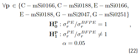
Where σ r is the standard deviation of the relative errors.
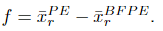
For the second hypothesis expressed in (23), the analysis method uses the two-sample t-test without the assumption of equal variances, which measures the distance between the two planes as follows,
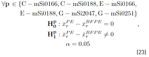
where the mean of the relative errors is expressed as ̄xr. In both hypothesis equations, the superscript PE means plane equation, and BFPE means best-fit plane equation.
7. Analysis and results
According to the results seen in Table 5 and Figures 4 and 5, it is clear to the authors that models with a high number of fitting parameters adjust the IEC efficiency data better. Table 5 shows the metrics for all PV modules, and the MPM represents better the behavior of the efficiencies derived from the power matrix. MPM models present the highest values of
 more than 99.5%, and the lowest values of nRMSD lower than 0.36% concerning the other models. It is seen that the efficiency values calculated from the IEC standard are better described by MPM, Durish, and HEY models than the proposed PE model. Actually, the proposed PE presents the worse fitting for the IEC data. However, when thousands of outdoor efficiencies are used, the PE model performs much better than the other parameter fitting models, as it is shown in Table 7. Notice that outdoor efficiency values are not taken at specific conditions (temperature, irradiance), as opposed to the case in which the IEC 61863-1 standard is used.
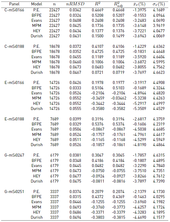
In Table 7, the nRMSD column presents results in the range of [3.15−5.55] %which represents how the outdoor efficiency values are scattered around the efficiency models. Notice that the plane-based models have the best-adjusted coefficient of determination,
 , i.e., the plane models capture much better the variability of the error than efficiency models calculated from IEC61853-1. In summary, the efficiency prediction model based on a plane in which parameters were calculated using a best-fit algorithm (BFPE) performs better than the model-based which parameters have been calculated using only three points (PE) or the other efficiency models: Evans, Hey, Durish, MPM. Nevertheless, as stated before, the three-point plane-based model is more practical due to the possibility of constructing it just with three reference values which may be taken from IEC references or data sheets without fitting procedures.
A relevant characteristic to consider is that the BFPE and PE models differ only by an offset value that is on average−1.94%as can be appreciated graphically in Figure 3. The displacement between the models is measured with the mean relative error ( ̄xr) and for the plane models do not vary significantly in all the modules analyzed (see Table 7].Actually, this displacement is observed in the histograms for the PE and the BFPE presented in Figure 6. In order to show a specific example, we selected the PV module C-mSi0166. The histograms in Figure 7 show the relative error distribution for both efficiency models. The results presented in this figure are confirmed in Table7 where it can be seen that the average of the relative error ( ̄xr) for the PE is−1.39%, while for the BFPE is−0.1533%,i.e., the difference between these averages is only1.24%.Therefore, the hypotheses established in (23) are rejected because those averages are not equal. On the other hand, the standard deviation of the r.e.(σr) presents similar results for both models indicating that the hypothesis in Equation (22) may be accepted or rejected.
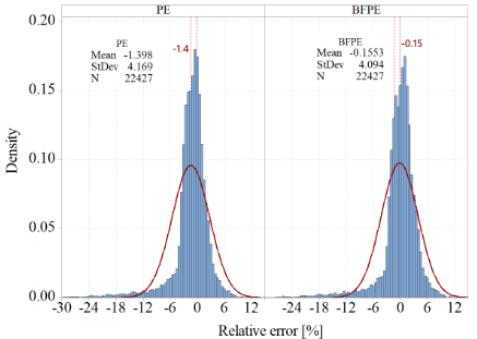
Figure 7 Histograms of the R.E. for panel C-mSi0166 a) r.e. distribution for the proposed equation b) r.e. distribution for the BFPE
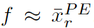
Based on observation of the previous results, we hypothesized that the three-point plane efficiency model could give the same prediction results as the best-fit plane model if the former is rewritten as,

where
The previous model (24) is called the adjusted plane equation (APE). Notice that according to Table 7
 is at least one order of magnitude smaller than
 and therefor
 . This equation means that if we multiply one PE model by a constant (1 +f) it is possible to displace the plane equation and obtain an equivalent plane to BFPE.
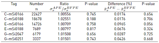
The new APE model has similar metrics to the BFPE model calculated from the outdoor data. For example, the nRMSD is almost the same for these two models and this can be observed in Figure 8. Notice that the APE model and the BFPE have the lowest nRMSD and could be considered equivalent models from the statistical point of view as we show next. Table 8 shows the results obtained when the hypothesis tests (22) and (23) are tested with the adjusted plane equation, where the P-Valued is the criteria used to accept or reject the null hypothesis H 0 .
The results in Table 8 are quite satisfactory. First of all, the standard deviation of the APE can be considered equivalent to the standard deviation generated by the BFPE. Second, both models generate an equivalent average of the relative error. It should be noticed that for all the tests made, the P-value is always higher than the acceptance value of 0.05; therefore, for all the six modules, it can be confirmed that both planes can be considered “parallel” and with equivalent error distributions.
8. Conclusions
This work has proposed a simple plane efficiency model to predict the efficiency value of PV modules using back-panel temperature and POA irradiance for outdoor conditions. The proposed PE model is calculated from three reference efficiency values obtained from the power matrix using the IEC 61853-1 standard. It was validated with outdoor efficiency values in three locations with data collected during one year. All the efficiency values data taken from the NREL database correspond to clean PV panels, with a temperature and irradiance in the ranges[25−65]° C and [200−1050] W/m 2 .
The proposed PE mode can be considered “parallel” to the best-fit-plane equation obtained from non linear regression of the efficiency data, and on average, the PE model is more optimistic with the predictions than the BFPE model. This means that the PE gives on average1.94%higher efficiency predictions for all the modules(f=−0.0194). However, when the PE is adjusted by the factor (1 +f), the adjusted plane equation generates, statistically speaking, equivalent results to the BFPE as demonstrated with the hypothesis test.
The usefulness of the proposed efficiency plane expression hinges on the possibility of constructing it with only three points. Even though a more accurate expression can be obtained by applying a best-fit algorithm to a set of measurements; these are not always available or desirable to obtain. A cloud of data, such as the one used in this paper for validation, requires measuring each PV module for months with high-precision equipment, which makes it impractical to determine the parameters of an efficiency model. Therefore, the main advantages of the proposed model are the simplicity of calculating the model constants and that the PE model describes the efficiency behavioral so like the best-fit plane efficiency model for a cloud of efficiency points, this without experiments nor data regression.

