


 English (pdf)
 Article in xml format
 Article references
 Send this article by e-mail
 Cited by SciELO
  Cited by Google
  Similars in
SciELO
Similars in
SciELO  Similars in Google
 Permalink
1. Introduction
Most communities in the world use stabilization ponds as a wastewater treatment method, almost always due to their attractive cost of operation. These lagoons are normally shallow excavations surrounded by earth slopes, with a rectangular or square appearance [1].
The overall performance of a wastewater treatment system depends on the effectiveness of the biokinematic processes and the hydrodynamic performance of its lagoons. In order to evaluate this last aspect, tracer tests are usually used. However, these experiments have been insufficient for an absolute understanding of the hydrodynamics of the system. In addition, this practice is influenced by external factors not considered such as environmental or meteorological [2].
Computational fluid dynamics (CFD) offers the option of simulating the hydraulic behavior of one or several fluids in a specific system, thus avoiding resorting to experimentation or preventing unwanted events during the process [3].
Previous studies [4-8] have demonstrated the ability of CFD to predict the behavior of the flow inside a facility, which makes it possible to evaluate the hydraulics of the system and detect inefficiencies that affect the process. To increase the efficiency of wastewater treatment systems, and thereby favor the removal of contaminants, many of these studies have considered the incorporation of physical restrictions (baffles) [3].
Baffle design can vary significantly, but these structures are typically floating, waterproof, and anchored at the base. They generally allow variable water levels and have low installation costs [9]. The main functions performed by the baffles are to increase hydraulic retention time (HRT), reduce hydraulic short-circuiting, and provide a submerged surface that can encourage the growth of adjoining biomass [10]. However, in other cases [11,12], baffles have not been found to increase HRT in stabilization ponds. Model studies have shown that certain flow conditions and baffle arrangements can inhibit mixing and reduce HRT. In particular, for very low flow velocities, baffles perpendicular to the direction of flow and ponds with a very high length-to-width ratio may have shorter HRTs as a result of the addition of hydraulic structures. Given this situation, other authors [13] emphasized the evaluation of the position and dimension of the baffles on the geometry of the pond.
Based on this analysis, two-dimensional studies were carried out on several modified proposals with baffles of a system of lagoons with variable length and width ratios. The results concluded that the configuration of baffles placed at 70 and 90% of the original size of the lagoon, obtained greater efficiency in pathogen removal [14].
2. Materials and methods
2.1 Stabilization Pond
The study was carried out at the wastewater treatment plant of the La Troncal canton, in charge of the drinking water and sewage company EMAPAT - EP, at coordinates: -2.407710910950- 09, -79.33729164878007.
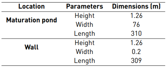
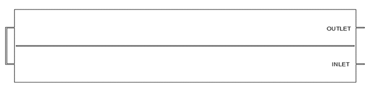
Figure 1 presents the pond modeled in this study, whose dimensions are shown in Table 1. The inlet and outlet conduits are located at medium depth and parallel, separated by a concrete wall. Between the slopes and the dividing wall, the formation of openings due to climatic and operational conditions over the years was detected, which in turn were included in the geometry to analyze their influence on the HTR.
2.2 CFD modeling
According to [11], a two-dimensional modeling of stabilization ponds has been a good alternative to three-dimensional modeling, due to its simplicity and computational economy. In addition, other authors have indicated that when modeling very shallow depths, there is little variation in the velocity profile at depth [15,16]. Therefore, a two-dimensional simulation of the MP shown in Figure 1 was performed using the ANSYS v.19.2 fluid dynamics software, with a second-order upwind numerical scheme and a SIMPLE pressure-momentum coupling.
Discretization of the domain
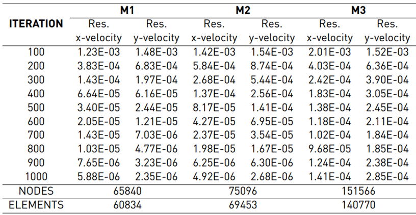
For this two-dimensional geometry, an unstructured mesh was created with the Quadrilateral Dominant mesh generation method, which prioritizes quadrilateral elements, and in conflicting areas, it is supplemented with triangular elements. As this study requires a greater level of detail in the analysis of the velocity and turbulence fields in the regions where these gradients are high, the incorporation of refinement was performed. A refinement of 0.01m was established for the inlet and outlet; the maximum element size was set at 3m, and for the edges of the walls and deflectors, three refinement sizes were tested: 1m for mesh 1 (M1), 0.5m for mesh 2 (M2) and 0.1m for the mesh 3 (M3).
Mesh independence analysis
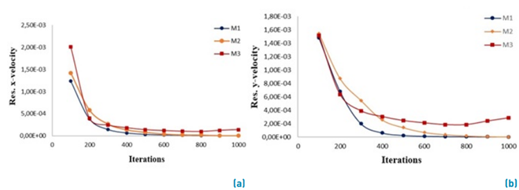
For the mesh independence analysis, single-phase steady-state hydrodynamic modeling of M1, M2, and M3 was performed. Then, the velocity residuals were plotted, both in the X and Y direction.
Table 2 shows the results of the steady-state modeling configured for 1000 iterations, and Figures 2a and 2b show the X and Y velocity residuals. From these plots, it can be interpreted that M1 and M2 have a lot of similarities, coinciding at certain points after 700 iterations. However, the residuals of M1 are very distant from M3, with M2 being the one that best approximates its behavior with the least number of elements.
Therefore, based on the computational demand that this entails, the mesh size configuration selected as optimal for this study was M2, which contains 69453 quadrilateral elements and an orthogonal quality and obliquity of 0.9632 and 0.2023, respectively, resulting in a high-quality mesh.
Standard model k-ε
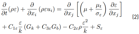
Since the flow regime is turbulent, for the stationary modeling of the velocity and turbulence fields, the standard k-ε model comprised by Equations (1) and (2) was used, which has been widely used in the modeling of stabilization ponds in CFD, with great success [2].
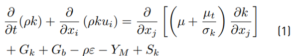
In these equations, G
k
represents the generation of turbulent kinetic energy due to mean velocity gradients. G
b
is the generation of turbulent kinetic energy due to buoyancy. Υ
Μ
represents the contribution of the fluctuating dilatation in the compressible turbulence to the total dissipation rate.
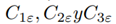 are constants. σκyσε are the Prandtl turbulence numbers for k and ε respectively.
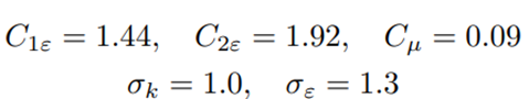
The constants presented in advance have the following default values:
Species transport model
There are two ways available to perform a virtual plotter test on CFD [17] . The first is to define a tracer (passive scalar) with the same properties as the study fluid; inject it at the input through the boundary conditions and monitor the concentration of this pseudo compound at the output. The second is to define solid particles that have the same density as the flowing fluid and a very small diameter, injecting a quantity large enough to obtain statistically significant results and observing the time it takes for each particle to leave the system. This study opted for the first alternative on the recommendation of a comparative study [18], which obtained a better fit for the experimental data.
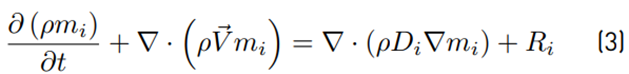
The equation for the conservation of mass for each chemical species i can be expressed in its mass fraction 𝑚 𝑖 , assuming that Fick's law holds [19].
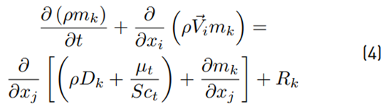
averaging Equation (3) for the case of turbulent flow, it comes to Equation (4):
Boundary conditions
An inlet velocity profile was applied based on the nominal flow rate of the pumping equipment, the daily operation time, and the dimension of the inlet duct. The residence time distribution (RTD) analysis was performed by applying a transient simulation of the tracer as a scalar on the velocity and turbulent fields obtained from the stationary simulation. The properties of the tracer material were defined identically to those of the primary fluid. The tracer was injected at time t = 0 s for one- time step, giving a mass fraction of 1, and then reset to 0 s for the second and subsequent time steps. The RTD was obtained by generating a surface report of tracer concentration versus time at the pond outlet [20].
RTD Analysis
Being MP a large reactor, it is evident to believe that the elements that make up the fluid take different times to cross the entire control volume [21]. These deviations arise because of channeling, recirculation, or the creation of stagnant areas. In order to analyze these phenomena, the performance of the residence time curves was used. The hydraulic parameters from the RTD curves are shown in Table 3.
SPulse curve
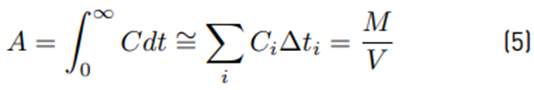
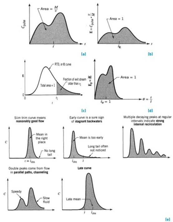
The reading of the tracer concentration at the outlet of a reactor as a function of time is also known as the Cpulse curve, expressed in kmol/m3 as shown in Figure 3a, where M represents the tracer concentration in kmol, v the fluid flow rate in m 3 / s, ̅t the mean residence time in days and V the volume in m 3 . From the mass balance for the reactor, the area under the curve (Equation (5)] and the mean of the curve (Equation (6)] are obtained.

E Curve
To find the E curve from the Cpulse curve, only the concentration scale had to be changed, so that the area under the curve is unity. This is achieved by dividing the concentration readings by
 , as shown in Figure 3b.
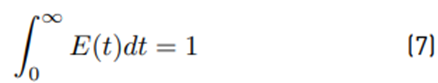
Equation (7) represents the mathematical normalization of the RTD function, where the fraction of the fluid that meets a duration of time t inside the reactor, is given by the value of E(t)dt.
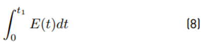
The fraction of the fluid that leaves the reactor with a duration less than is given by Equation (8) .
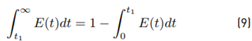
Also, the fraction of the fluid with a duration greater than t1 is obtained using Equation (9) and it is represented by the shaded area in Figure 3c.
Normalized E curve
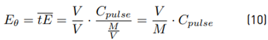
Finally, another RTD function was obtained, Eθ given by Equation (10). In this case, the time is measured as a function of the average residence time
 , as indicated in Figure 3d. For the characterization of the flow, dimensionless parameters of time θ and concentration were used Eθ, indicated in Figure 3e for plug-type flows [21].
Quantitative analysis of residence time distribution
Once the DTR curves were obtained, following a statistical procedure, some of the parameters that define the hydraulic analysis of the pond were determined [12]. Dead zones are recognized as those sectors where the flow remains stagnant or circulates slowly. Active volume is the opposite definition of a dead zone. The short circuit index indicates an inversely proportional relationship to the strength of the short circuit; a positive change refers to a decrease in the strength of the short circuit, and therefore an increase in the hydraulic performance, where S = 1 represents an ideal plug flow behavior. And the Persson hydraulic efficiency, which describes the uniformity of the flow distribution within the pond, where 1 represents ideality and values close to zero, unsatisfactory behavior [21].
3. Results and discussion
3.1 Stationary modeling of the MP
The velocity contours obtained by CFD in Figure 4 show the phenomena caused by channeling, recirculation, or the creation of stagnant zones. The color palette of Figure 4a relates the flow velocity in each sector of the pond, while the lanes followed by the current can be seen in Figure 4b and the preferred directions of flow are indicated in Figure 4c by vector superposition.
3.2 Transient modeling of the MP
Injection and transport of the virtual tracer
The transient modeling was divided into two parts: tracer injection and tracer transport. The tracer was injected at time t = 0 s for a time step, giving a mass fraction of species equal to 1, and then the mass fraction was reset to 0 for the following time steps. For the tracer injection, the number of time steps was 10 with a size of 0.1 s and for the tracer transport, the number of time steps was 172800 with a size of 1 s (48 h) with 1 iteration per time step. These time step values ensure the independence of the results. The residence time distribution was obtained by plotting the tracer concentration versus time at the pond outlet.
Figure 5a shows the virtual tracer concentration contours during one second of modeling. This process consists of the initial stage of the freezing method, or pulse experiment [18]. The subsequent stage indicated in Figures 5b-4e corresponds to the non-stationary modeling of the transport of the virtual tracer during a period of 4 days referred to the virtual environment, as a recovery criterion for most of the tracer.
The tracer distribution reveals the influence exerted by the opening in the wall next to the inlet. The flow recirculations in both blocks cover the entire length of the pond and make it impossible for the tracer to progress. As a result, there is a tracer available in low concentrations, but distributed over most of the pond, and especially over the return sector.
3.3 Analysis of RTD curves
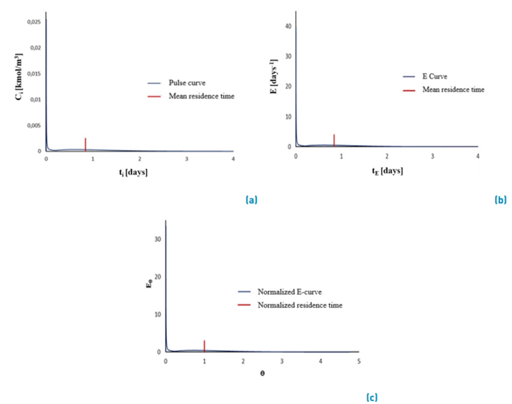
Figure 6a reports the shape adopted by the pulse curve, which revealed the reading of high tracer concentrations during the initial modeling stage, due to the presence of hydraulic short circuits; and between days 0.5 and 4, a notable reduction in the concentration read at the outlet of the unit was observed.
By converting the area under the curve to unity, it was required to know the fraction of fluid that leaves the pond during the stage that gives rise to the formation of the crest of the curve presented in Figure 6b. The reference duration was 10 hours. And under this criterion, it was determined that 34% of the fluid leaves the pond.
Figure 6c plots the location of the normalized retention time on the tail of the normalized E-curve; this behavior revealed the presence of stagnant zones and recirculation problems.
3.4 Quantitative analysis of RTD curves
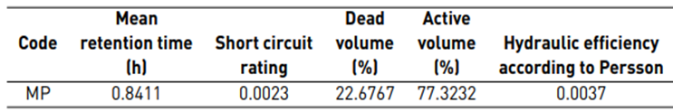
The first parameter found in Table 4 was the mean retention time, located in curve 5a on the elongated area of the tail. This phenomenon supposes the presence of stagnant zones where the CFD-simulated tracer slowly diffuses out of the MP [20].
The short-circuit index obtained reveals the presence of short-circuits, specifically in the inlet sector since S = 1 represents an ideal plug flow behavior, without the presence of short-circuits [11].
The high percentage of dead volume affects the importance of the location of the inlet and outlet conduit, as well as the dispersion dependent on the length-width ratio of the pond [22-24].
Finally, the hydraulic efficiency (λp) with a value that tends to 0, indicated a poor performance [25], as a result of the parallel relationship between the inlet and outlet of the pond.
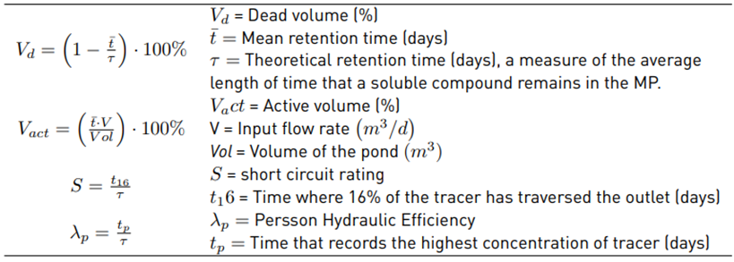
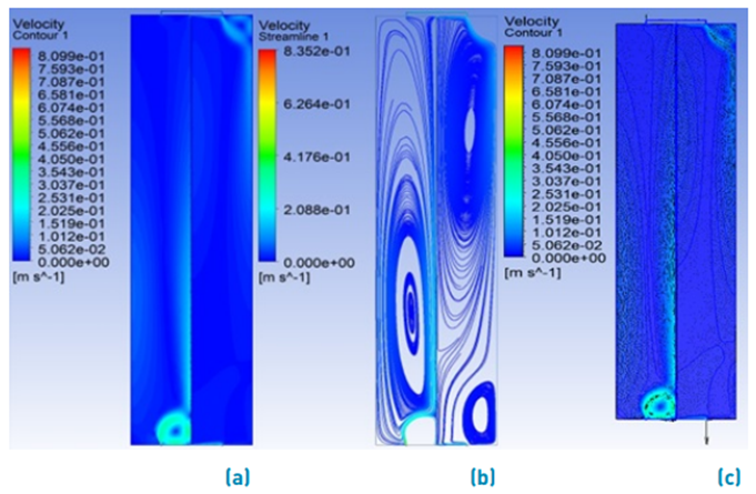
Figure 4 Contours generated from the stationary modeling for MP. a) Velocity contours. b) Velocity streamlines. c) Velocity Vectors plus contours
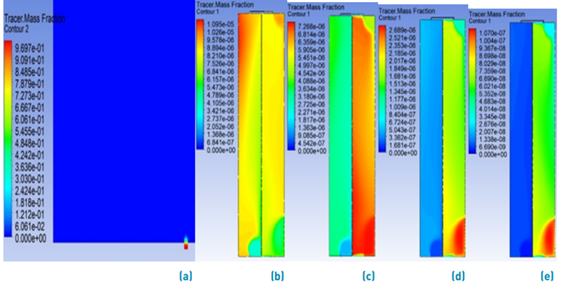
Figure 5 Tracer concentration across the pond as a function of modeling time. a) Virtual Tracer Injection b) After 12 hours of simulation. c) After 1 day of simulation d) After 2 days of simulation. e) After 4 days of simulation.
3.5 Optimization proposals
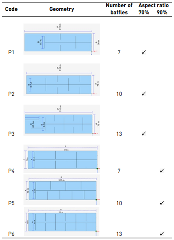
Having verified the hydraulic inefficiency of the MP and following the recommendation of previous studies carried out in stabilization pond systems, six modified geometric proposals were built with baffles configured at 70% [26], and 90% [14] in relation to the length and width of the pond.
In order to present a possible solution to carry out in practice, the arrangement of the inlet and outlet ducts was preserved. The opening between the lower slope and the dividing wall was closed, and the latter was transformed into a longitudinal deflector, as can be seen in Table 5.
3.6 Stationary and transient modeling for the modified proposals
Table 6 shows the flow streamlines obtained in the stationary modeling for the modified proposals with baffles, and the tracer concentration contours during the non-stationary modeling under the same MP modeling criteria. A mesh independence analysis for all these configurations (P1 to P6) was also carried out.
The geometrically modified proposals, except for P3, revealed the influence of the incorporation of deflectors on the successive transport of the virtual tracer; in addition, the hydraulic benefits of reducing recirculation to sectors can be visualized.
P3 indicates the formation of a stagnant zone between the upper left corner of the pond and the first longitudinal baffle. The placement of the longitudinal baffles at very short distances did not improve the progressive transport of the tracer for this case study.
3.7 RTD Analysis for modified proposals
Figure 7a shows the comparison of the surface profiles generated from the non-stationary modeling of the MP and the modified proposals. Two important aspects to highlight are the shape of the tail of the curve relevant to MP and the oscillations during the initial stage of tracer reading in P1. Previous investigations [15,27] indicate this behavior because of the presence of hydraulic short-circuits and recirculations, respectively. In this study, it is specifically reflected because of the opening in the wall in the case of MP, and the wide distance between the deflectors that make up P1.
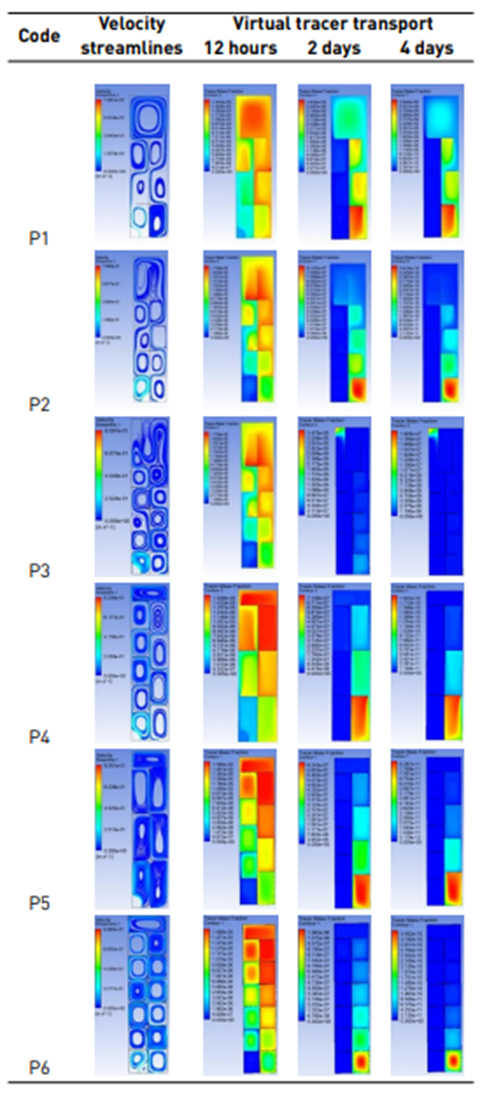
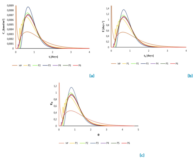
Figure 7 Comparison between the RTD curves of the MP and the modified proposals. a) Pulse curve. b) E curves. c) Normalized E curves
As indicated in the RTD analysis of MP, a useful characteristic of the E curve is to define the area under the curve as unity; this function allows analyzing the fraction of fluid that remains or leaves the reactor at the requested instant of time. For the cases of the modified proposals in Figure 7b, the reference age was the same as for MP. The results showed that fluid fractions of approximately 11% left the ponds P4, P5, and P6 in a common way, while the percentage of fluid dislodged for P1 was close to 15%. For their part, P2 and P3 reported dislodged fluid fractions equal to 5% and 9%, respectively, these being the most favorable results in terms of fluid retention during the initial test stage.
Through hydraulic characterization for plug-type flows [21] the phenomena immersed in the pond, described in Figure 3e, were predicted. Among the modified proposals, P2 and P3 better represent the behavior of a reactor that does not present anomalies, due to the location of the normalized mean retention time in relation to the crest of the curves. The formation of stagnant zones and recirculation problems become more noticeable for MP compared to the modified proposals and the influence of the distance between the baffles for P1 during the initial tracer reading is reiterated [Figure 7c).
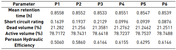
3.8 Quantitative analysis of the RTD curves for the modified proposals
The results shown in Table 7 show the similarity between the mean retention times of the proposals and MP, due to the tracer retention capacity on stagnant zones and elongated recirculations.
Among the proposals with 70% baffles, P3 has the best short-circuit index; and among the proposals with 90%, P4 presents the best index. The MP index is 92 times lower than P3, being the option that best approximates the ideal behavior plug flow.
Approximately 1% of the active volume was recovered by the inclusion of baffles. As mentioned above, the possibility of reducing stagnant areas depends essentially on the position and the number of inlets and outlets, which were preserved according to their origin in order to present a real optimization alternative to the treatment system.
The difference between the hydraulic efficiency of MP and the modified proposals shows the importance of closing the opening next to the inlet. Among the proposed cases, P5 achieved the best result, and among the configurations at 70%, only proposal P3 presented a result of interest. The efficiency of the P4 model has an intermediate value between P3 and P5; however, its construction volume is lower and, therefore, a cheaper option, due to its number of baffles.
4. Conclusions
The modified proposals with baffles at 90% in relation to length and width reported more favorable results in this study. Among the proposals modified at 70%, only P3 reported good results in terms of short circuit index and percentage of fluid retained during the first hours of simulation; however, the values obtained regarding the mean hydraulic retention time and active volume were unfavorable, compared to the proposals at 90%. Additionally, P3 has a greater construction volume due to the number of deflectors (13), which translates into a configuration that is not recommended in terms of costs. In relation to this last aspect, P4 is more viable than P5. As obtained in the analysis of the E curves, the percentage of fluid retained during the first hours of simulation for P4 and P5 were similar; this is not the case for the mean hydraulic retention time and short-circuit index, where the proposal with 7 baffles reported more favorable results. Finally, in terms of hydraulic efficiency, P5 stands out with a higher percentage, but not excessive compared to P4. Therefore, P4 was considered the optimal configuration among the options covered for this case study.

