


 English (pdf)
 Article in xml format
 Article references
 Send this article by e-mail
 Cited by SciELO
  Cited by Google
  Similars in
SciELO
Similars in
SciELO  Similars in Google
 Permalink
1. Introduction
Transportation Logistics was born and developed in association with human evolution. This is an essential need of current business development activities. When trade activities are being developed strongly, the demand for goods import and export increases which means that Transportation Logistics plays a more and more important role. Transportation Logistics accounts for more than 50% of cost and Logistics; economies are still constantly researching to optimize Transportation Logistics costs in the context of competition on a global scale. Particularly, during the Covid pandemic from December 2019 to the present, Transportation Logistics has increasingly demonstrated its role in transporting goods and maintaining supply chains on a global scale.
Road freight transportation is making an increase of Transportation Logistics activities, and has caused significant impacts on sustainability in the economies [1]. The major role of the transportation industry is not exclusively in an economic scope, but also as one of the leading fields generating the largest share of greenhouse gas emissions globally [2]. Transportation Logistics has many modes such as Road Transportation, Rail Transportation, Water Transportation, and Air Transportation, in order to transport each kind of cargo and human suitably [3]. Today, Transportation Logistics in terms of shipping activities is increasing and can cause potential hazards to commodities, the environment, and human lives [4]. The Transportation Logistics industry generates revenues from motor fuel taxes, vehicle registration, licensing, and parking and traffic which makes federal governments, the state, and the local community highly dependent on them [5].
Vietnam is a developing country in the Asian area. In 2020, despite the Covid-19 pandemic global spread, with a GDP growth rate of 2.9%, Vietnam is still one of very few countries in the world that has positive GDP growth. Ho Chi Minh is the largest trade city in Vietnam, which is the leading economic area of the country, and Ho Chi Minh’s GDP contributes roughly 25% of the national GDP annually. However, Transportation Logistics cost is one of the major barriers affecting the competitiveness of Vietnam’s economy. Transportation Logistics costs in Vietnam are equivalent to 20.9% of the GDP national country, a much higher rate than other countries in the Asian area, nearly two times higher than developed countries, and higher than the global average of 14%. The reason why transportation cost is too high which is equal to 30 - 40% of product costs, while this rate is only about 15% in other countries in the Asian region. Considering these reasons, a study in terms of Transportation Logistics’ development with the empirical case in Ho Chi Minh, Vietnam is necessary and valuable, to contribute to both Vietnam and the researchers related to this field.
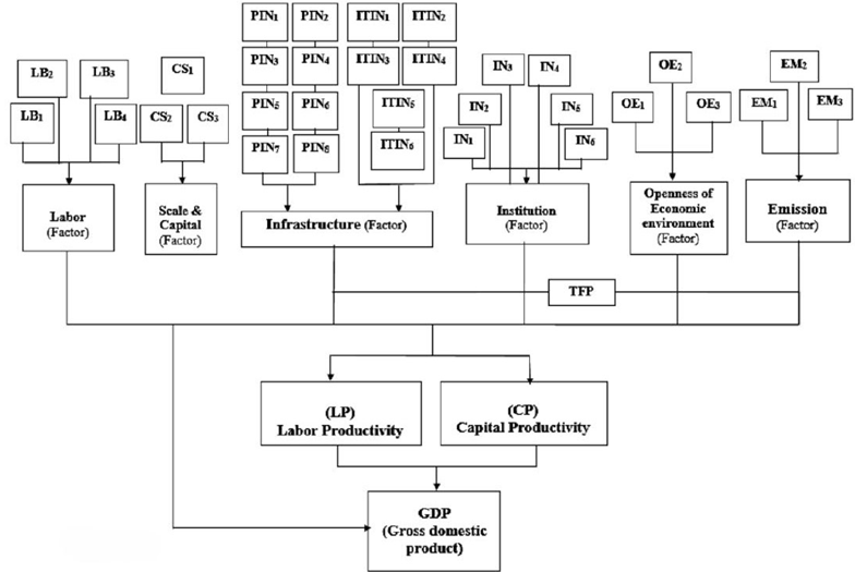
The objective of this paper is to measure seven factors. These are Labor, Capital & Scale, Physical Infrastructure, Information Technology Infrastructure, Institutions, Openness to the Economic Environment, and Emission. It also aims at assessing which factors impacts the Labor Productivity, Capital Productivity, and GDP of the Transportation Logistics Industry in Ho Chi Minh, Vietnam. Not everybody knows that Labor Productivity is the core of all factors that make up GDP. To improve Labor Productivity, it is necessary to create positive conditions to promote the Total Factor Productivity (TFP)’s growth rate. The Study model f this paper is developed based on the Cobb-Douglas production function. In this function, factor labor is studied by dividing it into four independent variables. These include female laborers, who have had a trained career, have graduated from high school, and have had a Labor index. Factor capital is divided into two independent variables consisting of business capital and fixed assets & long-term investment capital. Infrastructure, Institution, Openness to the economic environment, Emission belonging to TFP. This content is thought a novel contribution to this paper.
The paper has six sections, including: section 1 is the Introduction. Section 2 is the Literature review. Section 3 is the Methodology and Study Hypothesis. Section 4 is the Theoretical Basis. Section 5 is the Study Results. Section 6 is the Discussion and Section 7 is the Conclusion.
2. Literature review
We divided the Literature review into 2 parts including background theory and previous papers.
Background theory:
Cobb-Douglas production function:

As Equation (1) states:
P is the total production
L is Labor
C is Capital
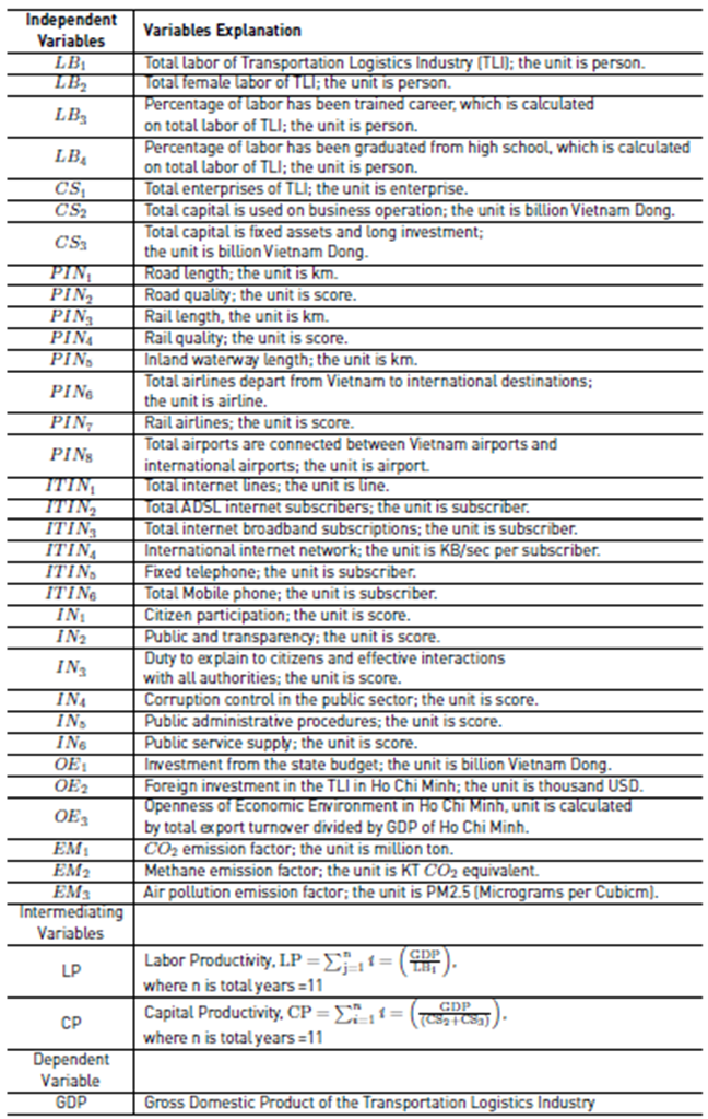
Labor and Capital are the basis for us to form two groups of variables LB and SC, in which labor is LB; LB includes four independent variables LB1, LB2, LB3, LB4, and SC is Capital including three independent variables SC1, SC 2, and SC3. Accordingly, we demonstrate the influence of Labor and Capital variables on the productivity and GDP of Transportation Logistics in HCM. Details are shown in Table 1.
The theory of TFP:

As Equation (2) states:
Q is the total output.
K is Capital.
L is Labor.
t is the occurrence of time in function F that allows “technical change”. “This is any type of change in the production function. Hence, the slowdown, the acceleration, the improvement in the education level of the workforce, are some variables included in this term” [6].
Accordingly, the theory of TFP focuses on the manufacturing industry. In this paper, we want to clarify the TFP of a service industry called Transportation Logistics through an empirical study in HCM, Vietnam.
Thus, function (2) will be:

As Equation (3) states:
PIN is Transport Physical Infrastructure
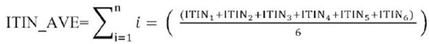
ITIN is Information Technology
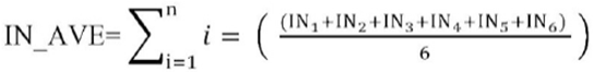
IN is Institutions
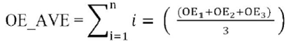
OE is Openness Business Environment
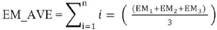
EM is Emission
PIN, ITIN, IN, OE, EM are independent variables belonging to t. In which, PIN includes 8 variables are PIN1, PIN2, PIN3, PIN4, PIN5, PIN6, PIN7, PIN8, ITIN includes 6 variables are ITIN 1, ITIN 2, ITIN 3, ITIN 4, ITIN 5, ITIN 6, IN includes 6 variables are IN 1, IN 2, IN 3, IN 4, IN 5, IN 6, OE includes 3 variables are OE 1, OE 2, OE 3, EM includes 3 variables are EM 1, EM2, EM 3. Details are shown in Table 1.
Previous papers:
[7] argued that “Sustainable investment policies increase the productivity of the gold mining system in Colombia. Increases of social capital promotion activities and physical infrastructure in the region of influence affect positively the multifactorial productivity of the Colombian gold mining process".
In terms of institutions, Regulatory frameworks play a vital role in Transportation Logistics [8]. The transportation sector’s regulatory frameworks are taxes, customs, and duties. Indeed, fuel taxes contribute to a significant portion of the revenue to the budget of governments. In the Transportation Logistics industry, technology can significantly reduce its costs, improving the quality of Transportation Logistics services [9]. The application of information technology German standard Richtlinien für den Lärmschutz an Straben (RLS 90) allows us to predict noise levels with good accuracy in areas where road noise prevails, which improves Transportation Logistics' quality [10] .
Industry scale and the covering level also play roles in Transportation Logistics, which are needed to integrate requirements of packing, and operating costs, assign orders to trips, and integrate the reverse flow of empty containers [11]. Transport infrastructure in China's Belt and Road Initiative countries plays an essential role in promoting economic growth [12]. The impact of the road and transport infrastructure of the China-Pakistan economic corridor is positively related to community support for tourism. In this sense, Tourism benefits have been perceived and the satisfaction of the community plays a role in this relationship. Pakistani local’s perception in terms of tourism due to road and transport infrastructure development in the China-Pakistan economic corridor [13].
Additionally, logistics transport infrastructure needs to have urgent attention to public spending’s impact on the labor share. Policy choices can be suggested to lessen the negative impact of road infrastructure on employment rates in China [14]. Using information technology such as the Frank-Wolfe algorithm demonstrates a positive effect on traffic flow, especially during rush hour causing traffic jams [15]. This is due to the difference between the CO2 emission factor of diesel [kg CO2/diesel gal] and biodiesel [kg CO2/biodiesel]. Consequently, to achieve a 230.81 kg CO2 reduction, 304 gallons of biodiesel should be used to replace the same amount of diesel on the market [16]. Information technology applications such as a Vehicular Ad-Hoc Network (VANET), Wireless Sensor Network (WSN) are increasingly needed to exchange information between vehicles and infrastructure to improve driving conditions in order to have a development of Transportation Logistics system [17]. The rapid expansion of the Transportation Logistics network greatly facilitates the movement and transmission of information between cities, which is very important in promoting the development of economic activities and reshaping the spatial model of economic geography [18]. In Tokyo, Japan, the property bubble occurred in the late 1980s and its aftermath led to drastic fluctuations in land prices affecting Transportation Logistics facilities [19]. Citizen participation affects the consideration of the difficulties of managing Transportation Logistics [20]. European Union countries have been improving their Transportation Logistics environmental performance between 2017 and 2018. For less efficient countries, improving Transportation Logistics sustainability is achieved mainly by reducing greenhouse gas emissions from fossil fuel-powered engines, increasing the share of freight transport by rail and inland waterways as well as the share of transport energy from renewable sources [21].
Transportation Logistics has a positive effect on business enterprise activities in the Mekong Delta region. In Vietnam, the degree of Logistics influence varies, depending on the business sector. In Vietnam, Logistics costs are considered the most important factor to improve the country's Logistics system. Therefore, it is necessary to reduce costs to achieve the optimal balance between costs and revenue [22]
In Vietnam, goods transportation’s demand, proximity to the market, production areas, customers, and transportation costs are considered the most important factors to determine the location of Logistics centers [23].
3. Methodology and study hypothesis
3.3. Sample collection method and data source
Sample collection method
Step 1: In theory, the templates are built based on the Cobb-Douglas production function and TFP theory. Accordingly, the Labor (LB) includes 4 independent variables and the capital (SC) includes 3 independent variables based on the Cobb-Douglas production function. TFP includes the Transport Physical Infrastructure (PIN) includes 8 independent variables, the Information Technology (ITIN) includes 6 independent variables, the Institutions (IN) includes 6 independent variables, the Openness Business Environment (OE) includes 3 independent variables, and Emission (EM) includes 3 independent variables. Details are shown in the Background theory of the Literature review.
Step 2: Cronbach's Alpha is used to test the reliability of the variables. Accordingly, variables that do not reach the Alpha scale will be eliminated to proceed to the step of Exploratory Factor Analysis.
Step 3: Exploratory Factor Analysis is used to measure and select variables. Thus, the selected variables are more significant than the excluded ones, but still contain most of the information content of the original observed variables.
Step 4: Pearson Correlation is used to measure the correlation between independent variables, intermediate variables and dependent variables.
Data source
Data is the secondary data of the time series from 2010 to 2020 collected by the authors by manual extraction from the Ho Chi Minh statistical yearbook, from the Ho Chi Minh Statistics Department, the General Statistics Office of Vietnam. From PCI of Vietnam Chamber of Commerce and Industry and United States Agency for International Development in Vietnam. From PAPI of the Center for Development Research and Community Support under the Vietnam Union of Science and Technology Associations and the United Nations Development Program in Vietnam. And from Thomson Reuters.
3.4. Study method
Step 1: Cronbach’s Alpha Test: to test the reliability of seven sets of observed independent variables; these steps include Labor, Capital & Scale, Physical Infrastructure, Information Techonology Infrastructure, Institutions, Openness of Economic Environment, and Emission.
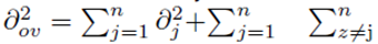
Cronbach's Alpha =
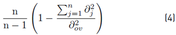
As Equation (4) states:
Where,
n is the total observed variables. In this paper; Factor Labor has n = 3. Factor Capital & Scale has n = 3. Factor Physical Infrastructure has n = 8. Factor Information Technology Infrastructure has n = 6. Factor Institutions has n = 6. Factor Openness of Economic Environment has n = 3. Factor Emission has n = 3. Details of all observed variables are described clearly in Table 1.
ov is observed variables


Step 2: Exploratory Factor Analysis (EFA): to measure and choose from many interdependent observed variables into a number of less observed variables which are called factors. Hence, the selected observed variables are more meaningful, but they are still contained most of the information content of the original observed variables.
In EFA, each measurable variable is represented as a linear combination of basic factors. Each measurable variable’s variability is explained by common factors. Measurable variables’ overall variability is described by some common factors, and an identified factor for each variable. The Equation below represents the factor model for the standard measure variables.

As Equation (5) states:
Where,
Xj is a measurable variable j has been normalized
ajn is the normalized multiple regression coefficient of factor n for measurable variable j
Y1, Y2, …, Yn are common factor 1, factor 2,…, factor n
Uj is the normalized regression coefficient of identified factor j for measurable variable j
Oj is an identified factor of measurable variable j
Identified factors are correlated with each other, and they have a correlation with common factors. The common factors are also described as linear combinations of measurable variables, measured by the following Equation:

As Equation (6) states:
Where,
Zj is an estimation of the coefficient of factor j
Wj is the coefficient weight of factor j
k is the total measurable variables
In this paper, after being tested by Cronbach’s Alpha, the following selected factors will have EFA one by one:
The Labor factor has four measurable variables;
The Capital & Scale factor has three measurable variables;
The Physical Infrastructure factor has eight measurable variables;
The Information Technology Infrastructure factor has six measurable variables;
The Institutions factor has six measurable variables;
The Openness of the Economic Environment factor has three measurable variables;
The Emission factor has three measurable variables.
Step 3: Pearson Correlation test: to measure the correlation between independent variables and intermediating variables, between independent variables and a dependent variable, and between intermediating variables and a dependent variable.
Pearson Correlation coefficient =
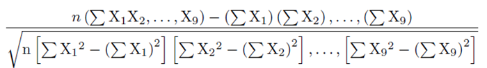
As Equation (7) states:
Where,
n is total variables, in this paper n = 9, which includes seven sets of independent variables, one set of intermediating variables, and one dependent variable
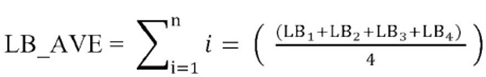
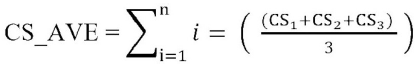
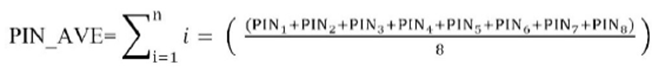
Seven sets of independent variables and one set of intermediating variables are calculated by average value, by the Equation below:
The average independent variable of Labor:
Average independent variable of Capital & Scale:
Average independent variable of Physical Infrastructure:
Average independent variable of Information Technology Infrastructure:
Average independent variable of Institutions:
Average independent variable of Openness of Economic Environment:
Average independent variable of Emission:
Average intermediating variable of Labor Productivity and Capital Productivity:
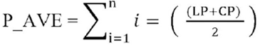
Where n is total years, n = 11
Step 4: Multivariate regression (MR)
Basic MR model:

As Equation (8) states:
Where, “a0” is the intersection between the vertical axis and the regression line.
“u” - where “u” is another factor beyond X1, X2, X3 ,…, Xn that this paper does not have analysis.
X1, X2, X3,.., Xn are independent variable 1, independent variable 2, independent variable 3,…, independent variable n.
In this paper, there are total of thirty-three independent variables, two intermediating variables, including Labor Productivity (LP) and Capital Productivity (CP), and one dependent variable GDP.
After being assessed by Cronbach’s Alpha, EFA, Pearson Correlation, each factor will have Multivariate regression with intermediating variable LP, intermediating variable CP, and dependent variable GDP, respectively.
Y = LB, CP, GDP, respectively.
X = independent variables of seven factors mentioned above, which are described clearly in Table 1.
According to [24] and [25], here,
ao + a1 + a2 + a3 +…+ an = 0 means that the regression model has not been built suitably to the input data and does not have statistical significance.
ao + a1 + a2 + a3 +…+ an ≠ 0 is to show that the regression model has been built suitably to the input data and it has statistical significance.
a1 + a2 + a3 +…+ an > 0 is to mean that independent variables have the same direction impact on dependent variable.
a1 + a2 + a3 +…+ an < 0 is to mean that independent variables have opposite direction impact on dependent variable.
How strong the impact of independent variables is based on their Beta coefficients.
3.5. Study hypothesis
H1: The independent variables have an impact on intermediating variable Labor Productivity and intermediating variable Capital Productivity.
H2: The independent variables have an impact on the GDP of the Transportation Logistics Industry.
H3: The intermediating variable Labor Productivity and intermediating variable Capital Productivity have an impact on GDP.
4. Theoretical basis
4.1. Female Labor
Participation of women in the workforce has been paid in numbers unprecedentedly in the 20th century [26] The world economy has identified trade as a potential determinant of female labor force participation. The female labor force increases whenever trade expands in areas where they employee a high number of female workers. Under conditions of high complementarity between capital and female labor, women's marginal productivity falls more than men’s. As a result, the gender wage gap widens and the female workforce decreases [27].
4.2. Transportation Infrastructure
Transport infrastructure consists of roads, railways, inland water, air transport, and maritime transport infrastructure. Transport policy and infrastructure itself are unified, which is one of the most important elements of the integration of individual European Union countries into one economically and socially efficient structure [28]. The development of the transportation infrastructure system should improve to increase its effectiveness and boost new unique transport, logistics and intelligent technologies [29].
4.3. Institutions
Institutions are man-made rules of interaction that constrains the opportunistic and volatile behavior of people. Institutions make the actions of individuals more predicTable. Institutions that want to be effective must include some forms of sanction for non-compliance [30]. Institutions have an impact on economic growth, it develops through two channels which are supporting more open and efficient markets, and supporting economic growth and poverty reduction. When the institutional structure does not encourage creative entrepreneurial talent, it encourages redistribution and rent-seeking which leads economic growth to be lower. Therefore, an institutional structure that encourages talent and creativity in production is extremely important for economic development [31].
4.4. Economic Environment and Emission
The empirical study in China [32] stated that “There is significant spatiotemporal heterogeneity between economic development and ecological environment. Economic development and ecological environment are in an intermediate coupling coordination stage, causing more regions to lag economically”. The costs incurred and the amount of pollutant emitted are roughly equal to the economic regulatory value [33] . The impact of GDP per capita growth on haze pollution has confirmed the relationship of the “inverted U” (Environmental Kuznets Curve). At the same time, urbanization has limited haze pollution, evidence of the existence of an Environmental Kuznets Curve between GDP per capita growth and haze pollution [34].
4.5. Transportation Logistics
Transportation Logistics is a key sector in developed economies; it is an essential catalyst for economic and social activities. However, it is important to emphasize the opposite impacts of this activity identified in economics as opposite externalities [35]. The development of Transportation Logistics has a relationship with the dynamics of economic growth in the countries of the Caspian-Sea-Coast [36]. As one mode of Transportation Logistics, Rail-truck intermodal transportation plays a vital role in freight transportation in North America. Therefore, it is crucial to ensure continuity and minimize the adverse impacts of disruption [37].
5. Study results
5.1. Cronbach’s Alpha
Table 2 presents the first testing Cronbach's Alpha. To check up, measure, select and reject independent variables are based on [38]. Cronbach's Alpha of ITIN = -.214, OE = .293, EM = .030, Labor = .553, Capital & Scale = .668 are all < 0.5, so they are all rejected. Cronbach's Alpha of IN = .680, PIN = .691, CS = .668 are accepted, EM = .553 is < 0.6 that can be temporarily acceptable.
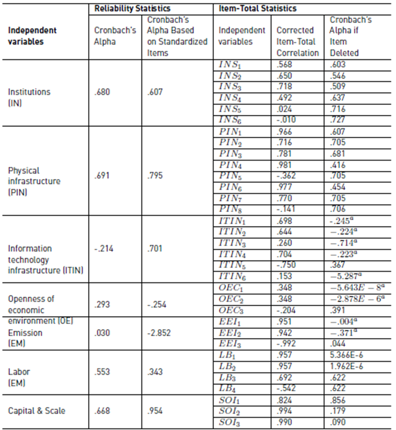
To check and reject Corrected Item-Total Correlation is based on [39]. Thereby, Corrected Item-Total Correlation of independent variables INS5 = .024 < 0.3, INS6 = -.010 < 0.3, PIN5 = -.362, PIN8 = -.141, LB4 = -.542 which are all rejected.
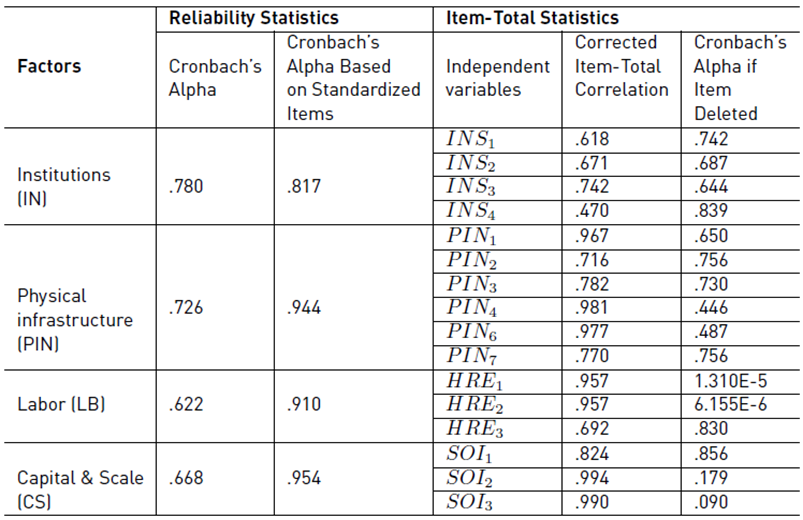
Table 3 gives us information on Cronbach’s Alpha testing result after ITIN, OE, EM, INS5, INS6, PIN5, PIN8, LB4 have been deleted, and Information Technology Infrastructure (ITIN), Openness of economic environment (OE) and Emission (EM) have been removed.
Cronbach’s Alpha of IN = .780, PIN= .726 are quite good. LB = .622, CS = .668 are both < .7 but they can be accepted.
Table 3 Cronbach’s Alpha testing result: after ITIN, OE, EM, INS5, INS6, PIN5, PIN8, LB4 have been deleted
Source: Study result of authors
In Exploratory Factor Analysis, one factor will be enough reliability if it has at least three observed variables [40,41]. Each selected factor in Table 3 has at least three observed variables.
About Corrected Item-Total Correlation, all items in Table 3 are > 0.3, which can all be kept. However, to have Cronbach’s Alpha be stronger, three items including INS4, PIN2, PIN7 have been removed.
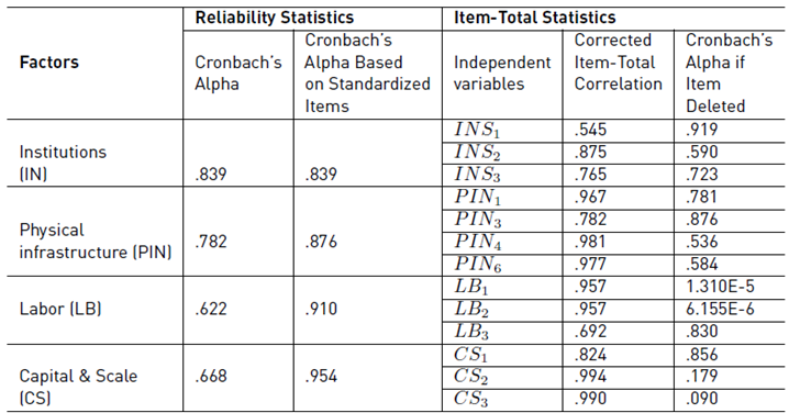
Table 4 illustrates Cronbach’s Alpha testing result after INS4, PIN2, and PIN7 have been deleted. Thereby, Cronbach’s Alpha of IN = .839, PIN = .806 are good and strong. Cronbach’s Alpha of LB = .622 and CS = .668, as explained in Table 3 that they cannot remove any more items, because LC and SC each have only three items.
Table 4 Cronbach’s Alpha testing result: after INS4, PIN2, and PIN7 have been deleted
Source: Study result of authors
The corrected Item-Total Correlation of all items in Table 4 is strong and > 0.3. All of them are accepted.
5.2. Exploratory Factor Analysis (EFA) results
Table 5 describes the result of EFA, KMO of PIN = .819 is good, KMO of LB = .660 is accepted. KMO of IN = .592, KMO of CS = .581 are thought as not good, but they can be acceptable.
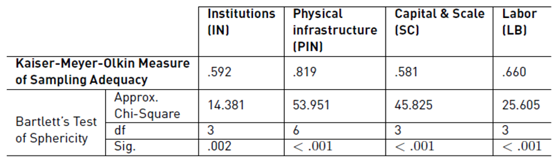
The standard of the EFA method is the KMO index must be > 0.5. And, the Barlett's test has a significance level of Sig < 0.05 to show the data used for factor analysis is appropriate, and observed variables are correlated with each other in the factor.
Sig Bartlett's Test: IN = .002, PIN < .001, SC < .001, LC < .001 which are all < .05 is to reject the hypothesis that observed variables are not correlated each other. Thus, the hypothesis that the correlation matrix between variables is homogenous is rejected, which is the variables are correlated with each other, and it is satisfied for EFA.
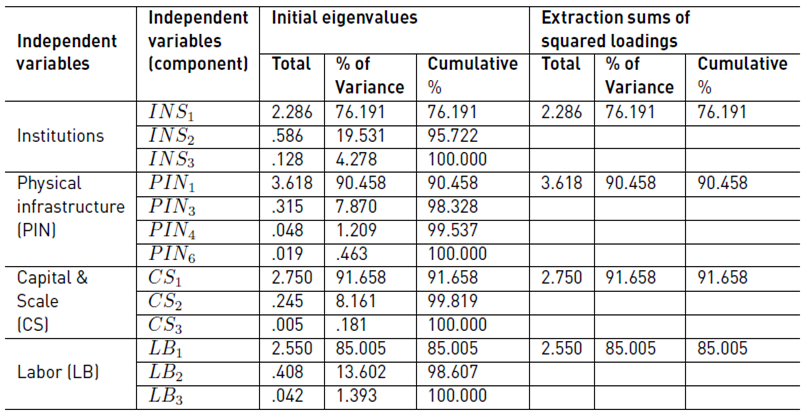
Table 6 presents the result of EFA by Principal components with Varimax rotation.
Three observed variables IN1, IN2, and IN3 of Institutions are initially grouped into one group.
Four observed variables PIN1, PIN3, PIN4, and PIN6 of Physical Infrastructure are initially grouped into one group.
Three observed variables CS1, CS2, and CS3 of Capital & Scale are initially grouped into one group.
Three observed variables LB1, LB2, and LB3 of Labor are initially grouped into one group.
Total variance of Institutions = 76.191% > 50%, it can be said that this factor can explain 76.191% of the variability of input data.
Total variance of Physical infrastructure = 90.458% > 50%, it is to mean that this factor can explain 90.458% of the variability of input data.
Total variance of Capital & Scale = 91.658% > 50%, %, it is to determine that this factor can explain 91.658% of the variability of input data.
Total variance of Labor = 85.005% > 50%, which is to understand that this factor can explain 85.005% of the variability of input data.
The Eigenvalues of Institutions = 2.286, Physical Infrastructure = 3.618, Capital & Scale = 2.750, Labor = 2.550 which are all high (>1).
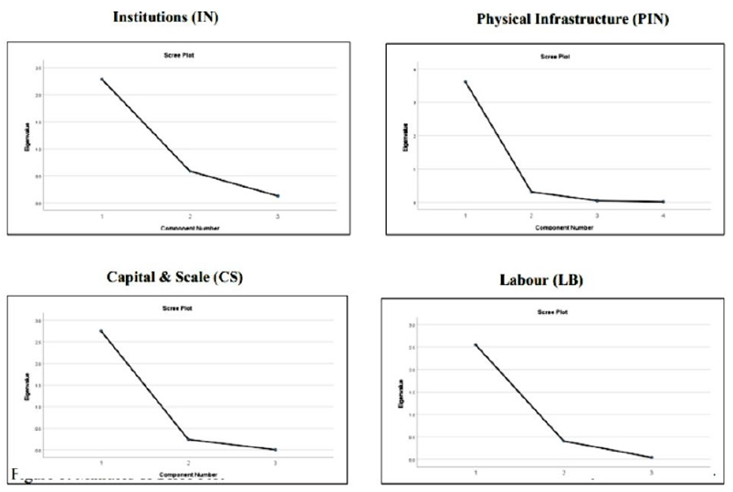
Figure 1 illustrates factors that have been selected by the Varimax rotation method with the appropriate number of factors that are presented in Table 6.
5.3. Pearson correlation
Table 7 describes the Pearson Correlation results. The authors evaluate three correlations below:
The correlations between two intermediating variables Labor productivity (LP) and Capital productivity (CP) by calculating the average value of LP & CP (LP&CP_AVE) with four sets of independent variables by calculating the average value. Four sets independent variables include Institution (IN_AVE), Physical Infrastructure (PIN_AVE), Capital & Scale (CS_AVE), Labor (LB_AVE).
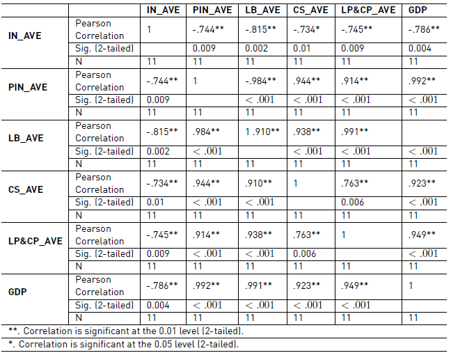
The correlation between the dependent variable GDP and four sets of independent variables IN_AVE, PIN_AVE, CS_AVE, LB_AVE.
Correlation between dependent variable GDP and intermediating variable LP&CP_AVE.
Sig. of intermediating variable LP&CP_AVE in correlation with four sets independent variables IN_AVE, PIN_AVE, LB_AVE, CS_AVE are 0.009, <.001, <.001, 0.006, respectively. They are all < .05, which is to show they have a correlation with each other.
Sig. of dependent variable GDP in correlation with four sets independent variables IN_AVE, PIN_AVE, LB_AVE, CS_AVE are 0.004 < .001, <.001, <.001, respectively. They are all < .05, which is to determine that they have a correlation with each other.
Sig. of GDP in correlation with intermediating variable LP&CP_AVE is < .001, and is < .05, is to understand that they have a correlation with each other.
5.4. Multivariate regression (MR) results
Table 8 presents the result of MR between independent variables Capital & Scale and intermediating variable Labor Productivity. R= .995, R Square = .990, Adjusted R Square = .985 is mean that the MR model is built at high reliability, which also indicates that input data has been explained by regression output at 98.5%. ANOVA has Sig. <.001 is to show the MR model has statistical significance at a level is < .001.
Table 8 Multivariate regression result between Capital & Scale and Labor Productivity
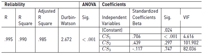
Source: Study result of authors
Durbin-Watson = 2.672, which is 1 < 2.672 < 3 to mean there is no Autocorrelation [42].
SC1 has Standardized Coefficients Beta = .706, Sig. <.001 and VIF of SC1 = 4.616 < 10 showing that there is no Multicollinearity. So, CS1 has the same direct impact on Labor Productivity at Beta = .706.
CS2 has Sig. = .297 > .05, VIF = 101.902, CS3 Sig. = .747 > .05, VIF = 82.036, which is show that there are Multicollinearities [43]. Hence, these results of CS2 and CS3 are not reliable.
Table 9 illustrates the MR results between independent variables Capital & Scale and intermediating variable Capital Productivity. R= .985, R Square = .971, Adjusted R Square = .959 means that the MR model is built at high reliability, and input data has been explained by regression output at 96%. ANOVA has Sig. <.001, that is to show MR model has statistical significance at a level is < .001.
Table 9 Multivariate regression result between Capital & Scale and Capital Productivity
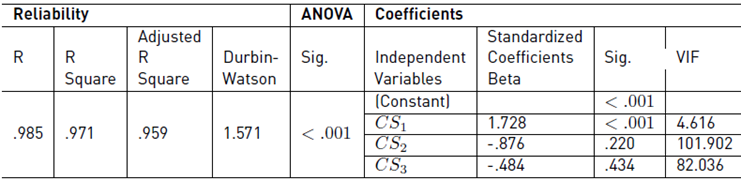
Source: Study result of authors
Durbin-Watson = 1.571 is between 1 and 3. Which is to show there is no Autocorrelation.
CS1 has Sig. < .001 and Standardized Coefficients Beta = 1.728, and VIF of CS1 = 4.616 < 10 is meant that there is no Multicollinearity. Hence, CS1 impacts in the same direction on Capital Productivity at Beta = 1.728.
CS2 has Sig. = .220, VIF = 101.902 > 10, and CS3 has Sig. = .434, VIF = 82.036 > 10, there are Multicollinearities. Hence, the result of CS2 and CS3 are not reliable.
Table 10 describes the Multivariate regression result between independent variables, Physical Infrastructure and intermediating variable Capital Productivity. R= .947, R Square = .897, Adjusted R Square = .828 shows the MR model has been built at high reliability, and input data has been explained by regression output at 83%. ANOVA has Sig. = .004, which means the MR model has statistical significance at level = .004.
Table 10 Multivariate regression result between Physical Infrastructure and Capital Productivity
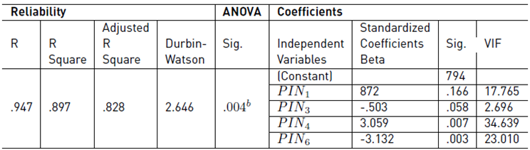
Source: Study result of authors
Durbin-Watson = 2.646, as 2.646 > 1 and 2.646 < 3, so there is no Autocorrelation.
PIN3 has Sig. = .058 > .05 which nearly has statistical significance, so it can temporarily be accepted, VIF of PIN3 = 2.696 < 10 means there is no Multicollinearity. Hence, PIN3 has an impact on Capital Productivity in the opposite direction at Beta = -.503.
PIN6 has Sig. = .003 < .05, VIF = 23.010 > 10, PIN4 has Sig. = .007 < .05, VIF = 34.639 > 10, PIN1 has Sig. = .166 > .05, VIF = 17.765 > 10, all have Multicollinearities. Hence, the results of PIN6, PIN4, PIN1 are not reliable.
Table 11 describes MR results between independent variables Capital & Scale and dependent variable GDP. R= .998, R square = .996, Adjusted R Square = .995 which means the MR model is built at high reliability, and to mean that input data has been explained by regression output at a perfect level of 99.5%. ANOVA has Sig. < .001 which means the MR model has statistical significance at level < .001.
Table 11 Multivariate regression result between Capital & Scale and GDP
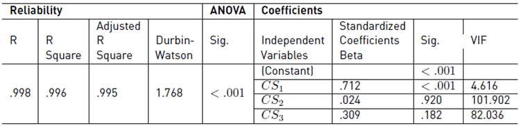
Source: Study result of authors
Durbin-Watson = 1.768 which is 1.768 > 1 and 1.768 < 3, that means there is no autocorrelation.
Independent variable CS1 has Sig. <.001, Standardized Coefficients Beta = .712, VIF = 4.616 < 10 which means there is no Multicollinearities. So, CS1 impacts on GDP in the same direction at beta = .712.
CS2 has Sig. = .920 > .05, VIF = 101.902 > 10, and CS3 has Sig. = .182 > .05. VIF = 82.036 >10 is show there are Multicollinearities. So, these results of CS2 and CS3 are not reliable.
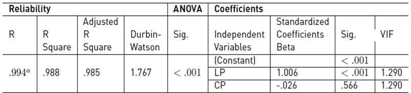
Table 12 illustrates the MR results between intermediating variable Labor Productivity, variable Capital Productivity, and the dependent variable GDP.
Table 12: Multivariate regression result between Labor Productivity, Capital Productivity, and GDP.
Source: Study result of authors
R= .994, R Square = .988, Adjusted R Square = .985 is to show MR model is built at high reliability, and input data has been explained by regression output at a high level of 98.5%. ANOVA has Sig. < .001 is mean MR model has statistical significance at level < .001.
Durbin-Watson = 1.767, as 1.767 > 1 and 1.767 < 3, so there is no autocorrelation.
There are only Labor Productivity (LP) impacts on GDP at Sig. <.001, Standardized Coefficients Beta of LP = 1.006, which is to show LP impacts on GDP in the same direction at Beta = 1.006. Capital productivity (CP) has Sig. = .566 > .05 is mean that there is no statistical significance, or it can be said CP does not impact on GDP.
VIF of LP = 1.290 < 10 and VIF of CP =1.290 < 10. So, there is no Multicollinearity.
6. Discussion
Based on study results in section 5, we have Cronbach’s Alpha results after testing three times. There are three sets of independent variables that have been removed. The result indicates Cronbach’s Alpha of Institutions = .839, Information Technology Infrastructure = .806, Labor = .622, Capital & Scale = .668. These four sets of independent variables that have been assessed by Exploratory Factor Analysis with the results are KMO of PIN = .819 is good, IN = .592 and LB = .660 are accepted, CS = .581 is thought to be not as good, but it can be accepTable. Sig Bartlett's Test of all these four sets IN, PIN, LB, SC are < .05 which means to reject the hypothesis that observed variables are not correlated with each other.
Principal components with the Varimax rotation method, include the Institutions factor that has three independent variables INS1, INS2, and INS3. The Physical infrastructure Factor has four independent variables PIN1, PIN3, PIN4, and PIN6. The Capital & Scale Factor has three independent variables CS1, CS2, and CS3. The Labor Factor has three independent variables LB1, LB2, and LB3 which are initially grouped into one group per each, respectively.
The total variance of these four sets, consisting of Institutions = 76.191%. Physical Infrastructure = 90.4581%. Capital & Scale = 91.658%. Labor = 85.005% which are all > 50%. These mean that factors IN, PIN, CS, LB can explain 76.191%, 90.4581%, 91.658 and 85.005% of the variability of the input data, respectively.
The Sig. of Pearson Correlation testing between LP&CP_AVE and four sets of independent variables IN, PIN, CS, and LB are 0.009, <.001, <.001, 0.006, respectively. Between GDP and four sets of independent variables are 0.004, <.001, <.001, <.001, respectively. Between GDP and LP&CP_AVE is < .001. These figures are to show that they correlate with each other.
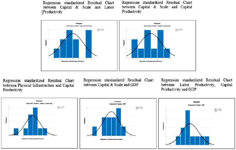
Multivariate regression results of five models have shown that R, R Square, and Adjusted R Square are at high reliability which Adjusted R Squares are from 83% to 99.5%. ANOVAs of four models have Sig. < .001, there is one model that has Sig. = .004; these are to prove that five Multivariate regression models have been built at high reliability, which is to show the input data are appropriate to the models, and have high statistical significance. There is no Autocorrelation in all models. Although Multivariate regression models are built at a high statistical significance and high reliability, and there is no Autocorrelation, there are Multicollinearities in three independent variables that have Sig. > 0.5, in two independent variables have Sig. < 0.5. Hence these results are not reliable and have been rejected.
Multivariate regression results
The multivariate regression result between intermediating variable Labor Productivity, intermediating variable Capital Productivity, and dependent variable Transportation Logistics Industry GDP: While intermediating variable Labor Productivity impacts in the same direction on GDP at beta = 1.006 and Sig. <.001, intermediating variable Capital Productivity does not impact on GDP at Sig. = .566 > .05.
CS1 is the independent variable, which is the total number of enterprises of the Transportation Logistics Industry: Multivariate regression’s result between independent variables Capital & Scale and Transportation Logistics Industry GDP shows independent variable CS1 has Sig. <.001, Standardized Coefficients Beta = .712, VIF = 4.616. Hence, CS1 impacts on Transportation Logistics Industry GDP in the same direction at beta = .712.
The Multivariate regression’s result between independent variables Capital & Scale and Labor Productivity shows that .
CS1 has Standardized Coefficients Beta = .706 and Sig. <.001 and VIF = 4.616, that is to say, CS1 has the same direct impact on Labor Productivity at beta = .706.
The result of the Multivariate regression between Capital & Scale and Capital Productivity shows CS1 impacts in the same direction on Capital Productivity at Beta = 1.728, Sig. <.001 and VIF = 4.616.
Multivariate regression result between Physical Infrastructure and Capital Productivity: PIN3 has Sig. = .058 > .05 which is nearly has statistical significance, so it can be temporarily accepted, VIF of PIN3 = 2.696 < 10. Hence, PIN3 has an impact on Capital Productivity in the opposite direction at Beta = -.503, PIN3 is Rail length.
Managerial implications
Based on the study results and discussion, the authors have policy implications, including:
First, since Labor Productivity affects the GDP of Transportation Logistics in the same direction, attention should be paid to increasing Labor Productivity as much as possible.
In addition, the total number of enterprises in Transportation Logistics has a positive impact on GDP of Transportation Logistics, on Labor Productivity, and on Capital Productivity. Therefore, managers and policymakers should focus on encouraging an increase in the number of businesses operating in the field of Transportation Logistics.
Moreover, in the planning and management policy mechanism, it is not necessary to care about Capital Productivity because Capital Productivity does not affect the GDP of Transportation Logistics.
Besides, PIN3 (Rail Length) has Sig. = .058 > .05 is close to statistical significance and should be temporarily accepted, Rail Length has an impact on Capital Productivity in the negative direction. Therefore, for the management and policy-making of Transportation Logistics, there should also be attention to minimizing the Rail Length.
7. Conclusion
Based on the study results in section 5, and the discussion in section 6, some remarkable findings are:
There are four sets of independent variables Instituion, Physical Infrastructure, Labor, and Capital & Scale factors that have been chosen in a total of seven sets of independent variables. Three sets of independent variables including Information Technology Infrastructure, Openness of Economic Environmment, and Emission have been rejected after being tested by Cronbach’s Alpha.
The Institution factor has Cronbach’s Alpha = .839 at a good reliability level after rejecting three independent variables from a total of six variables. Also the Institution factor has the KMO of Exploratory Factor Analysis = .592 at an accepTable level, and Pearson Correlation testing has Sig. = 0.009 in a correlation with Institutions, and Labor & Capital productivity, Sig. = 0.004 in a correlation between Institutions and GDP. These show Institutions has a correlation with Labor & Capital Productivity, and GDP. There is no variables impact on Labor Productivity, Capital Productivity and GDP.
Multivariate regression results have no Autocorrelation.
After Multicollinearities are rejected in all results of Multivariate regressions. The final results are; Regarding factor Capital & Scale, there is one independent variable, which is called the total number of enterprises in the Transportation Logistics Industry.
This impacts in the same direction on Labor Productivity at Sig. <. 001 and Beta = .706, it impacts Capital Productivity in the same direction at Sig. <. 001 and Beta = 1.728, and it impacts on Transportation Logistics Industry GDP in the same direction at Sig. <. 001 and Beta = .712.
In terms of Physical Infrastructure factor, there is an independent variable PIN3 (PIN3 is Rail Length) which has Sig. = .058 > .05, Sig. = .058 nearly having statistical significance. The authors consider it can provisionally be accepted, VIF of PIN3 = 2.696 < 10 which means there is no Multicollinearity. Hence, Rail Length has an impact on Capital Productivity in the opposite direction at Beta = -.503.
Finally, the Multivariate regression result between the intermediating variable Labor Productivity, the intermediating variable Capital Productivity, and the dependent variable Transportation Logistics Industry’s GDP shows that while intermediating variable Labor Productivity impacts in the positive direction on GDP at beta = 1.006 and Sig. <.001 VIF = 1.290, intermediating variable Capital Productivity has at Sig. = .566 > .05 which shows that there is no statistical significance, or it can be said that Capital Productivity does not impact GDP at Sig. = .566 > .05 VIF = 1.290.
Therefore, in order to develop accurately Transportation Logistics Industry, it needs to focus on Transportation Logistics Industry’s GDP. On the one hand, based on the theory that as we all know, Labor Productivity is the core of all factors that make up GDP. On the other hand, the result of this study is to prove that Labor Productivity impacts on Transportation Logistics Industry’s GDP in the same direction as Sig. <.001 and beta = 1.006. Thereby, in order to develop Transportation Logistics Industry, this industry needs to boost the GDP of the Transportation Logistics Industry by boosting its Labor Productivity. In particular, as total number enterprises of Transportation Logistics Industry impacts on Transportation Logistics Industry’s GDP in the same direction at Beta = .712. So in order to boost the GDP of Transportation Logistics Industry, it needs to consider and re-organize the Scale of the Transportation Logistics Industry in the direction of increasing the number of enterprises.
Besides, the independent variable total number of enterprises in the Transportation Logistics Industry impacts positively Labor Productivity at Beta = .706. Hence, it is more evidence to emphasize that the independent variable total number of enterprises of the Transportation Logistics Industry must be considered, re-organized and improved increasing the number of enterprises.
Limitation
The study results have not shown the authors’ expectations. The study model has been built which has seven factors, including seven sets of independent variables, two intermediating variables, and one dependent variable. There has been strictly tested step by step by Cronbach’s Alpha, Exploratory Factor Analysis, Pearson Correlation, and Multivariate regressions. The final results show that there are only two sets of independent variables which impact on intermediating variable Labor Productivity, intermediating variable Capital Productivity, and the dependent variable Transportation Logistics Industry’s GDP.
Authors plan to do the next study on this topic but using a different method to improve the research result.

