




 English (pdf)
 Article in xml format
 Article references

 Automatic translation
 Send this article by e-mail
 Cited by SciELO
 Cited by Google
 Similars in
SciELO
 Similars in Google

 Permalink


Introduction
Transit crashes are a topic of worldwide interest, due to their implications, such as the number of deaths, individuals injured with trauma, or individuals with permanent disabilities. These implications constantly limit the physical, psychological, and social well-being of citizens, decreasing their quality of life1,2. One of the most shocking statistics from the Global Status Report on Road Safety 20183 states that road traffic injuries are the leading cause of death among people aged 5-29 years.
The transit crash constitutes one of the most serious threats to the sustainable development of countries. In 2020, the Global Plan for the Second Decade of Action for Road Safety was promulgated, so that the member countries of the United Nations would adopt measures that would help reduce the number of deaths and serious injuries caused by traffic crashes to 50% by 20304.
Despite the efforts of national and international governments, there are high levels of incidence and a huge economic and social impact on countries and families of the injured5. It should be considered that there are different factors involved in a transit crash, ranging from environmental, control, and road supervision factors, extending to drivers and pedestrians, ending with moving vehicles6,7. The multicausal origin and the scarcity of specific analytical studies, accentuate the complexity of the approach to transit crash and possible prevention strategies8.
According to the French Road Safety Observatory9, traffic crashes have increased considerably since the early 1950s, in direct relation to the expansion of the number of vehicles, which in turn has been accompanied by the lack of suitable road networks and insufficient driver training. In addition to the increase in the number of people injured in traffic accidents and the neglect of governmental actions, it has become a public health problem10. In some countries, such as the case of the Colombian government, despite having declared road safety a state policy, and implementing measures in institutional, budgetary, regulatory and research matters, traffic accident rates continue to be high11, disturbing security, order and road mobility12.
In Ecuador, transit crash is a major economic, social and public health problem, as they are one of the main causes of death. As a result, Ecuador is one of the countries with the highest mortality rates for this type of accident in Latin America13. In this sense, it is expected that the State and the Ecuadorian economy will assume a high cost in hospital care and repair of damages caused by traffic crashes.
The Traffic and Mobility Agency (TMA) of Guayaquil presents annual statistical reports on road safety and traffic fatalities on its website; however, there is no open data on local traffic accidents within its geographical area of action. According to the National Transit Agency of Ecuador (NTA), the highest traffic control agency in the country, in the parish of Guayaquil, the total number of traffic accidents dropped from 4,989 in 2017 to 4,416 in 2021, with a reduction in the number of accidents. Still, unfortunately, the total number of "deaths in situ" went from 154 to 206. It should be noted that the city of Guayaquil has more than 2,723,665 inhabitants, according to 2010 census projections. More than 85% of the total population of the province lives in this city. It is grouped administratively into sixteen urban parishes that make up the aforementioned city14.
The few actions that have been taken on traffic issues are made on the basis of accident reports, after the fact, being applied in most cases, only to find culprits and assess damages6,7. It is estimated that the global burden of disease from road traffic injuries will continue to increase steadily; therefore, the development of a proposal to mitigate the risks of road traffic injuries will require an understanding of the complex interaction of the factors that lead to an accident 15.
These facts demonstrate why it is essential to know the causes of accidents by type. It must be based on reliable statistical models that establish the frequency of occurrence of traffic crashes and how they relate to the particular characteristics and situations of the incidents16, as well as multicriteria optimization methods7.
On the other hand, open data initiatives are rising in many countries. In 2022, Ecuador government issued “The open data policy”, through the agreement signed by the Ministry of Telecommunications and Information Society17. The objective of this policy is to promote the divulgation, use and reuse of open data. It is important to remember that the more rigorous the data sources used, the higher the accuracy of the analysis and results, the more detailed and reliable they will be. Facilitating appropriate decision making. 18. The data studied were taken from the open database provided by the NTA of Ecuador, which has as a source all the control institutions that have or have assumed competence in the operational control of traffic at the national level19.
The aim of this study was to provide a quantitative characterization of traffic accident data in Guayaquil, Ecuador, for the period from 2017 to 2022. In order to achieve this, descriptive and predictive statistical models were used in the analysis of time-series data related to accident rates and their outcomes.
These findings would aid in formulating programs to mitigate the risks associated with these incidents. The results of this type of study provide the opportunity to develop holistic road safety strategies that address the multilevel determinants of traffic accidents20. In addition, to give support in the design, implementation and evaluation of local and national intervention proposals. 21.
Literature review
2.1. Background
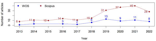
In order to evaluate the academic and scientific interest regarding the analysis of transit crash through applied statistics, a search was made on the indexed open-access articles in the high-impact databases Scopus and Web of Science (WoS), in which the terms "traffic accidents" and "time series" were used for the queries, within the period from 2013 to 2022, criteria applied to the title, abstract and keywords of the scientific production. These results were exported to perform the processing of bibliographic data. Firstly, the 205 documents found in Scopus report an annual growth of 14.93% in scientific production, and in WoS the 45 articles report an annual growth of 25.99%, see Figure 1.
The following is a chronological list of some of the research works, from the last three years of the period consulted in the databases, which have some similarities with the work developed, which served as evidence that the topic under study is of global interest and serves as a reference or guide.
The study developed for the Istanbul Police Department in Turkey, aims to determine the distribution of accident density in the regions using data from three years (2015, 2016 and 2017), to establish the causes of accidents and provide solutions22.
Likewise, the study done using data from the traffic police office of Oromia region of Ethiopia, recorded daily traffic accidents from July 2016 to July 2017. They used count regression models to analyze the factors associated with the number of human fatalities due to recorded daily on traffic accidents23. In a different research, an accident prediction model was developed for Hisar and Haryana in India, in which a comparative analysis of traffic accident data from these cities was carried out24.
In the specific case of Pakistan, temporal patterns have been created to forecast traffic crash rates by using univariate time series analysis, such as seasonal autoregressive integrated moving average (SARIMA) and exponential smoothing (ES) models. Some of the main results of the study were that the ES model was a better fit for the accident data than the SARIMA model after calculating the lowest mean absolute error, mean square error, mean absolute percentage error and normalized Bayesian information criterion25.
Similarly, a study was developed to determine the best model for forecasting traffic fatalities in Malaysia. The autoregressive integrated moving average (ARIMA) model and the autoregressive Poisson model were used. The results indicated that the best model was ARIMA (0,2,1), as it had a lower error measure compared to the autoregressive Poisson model26.
Regarding the research developed in the city of Belgrade, Republic of Serbia, the pattern of traffic crashes with time series was investigated. For this purpose, the data were described and understood from the exploratory data analysis through the regression method and Box-Jenkins autoregressive seasonal autoregressive integrated moving average model (SARIMA). It was found that the time series had a marked seasonal character. The model had a mean absolute percentage error (MAPE) of 5.22 % and could be seen as an indicator that the forecast was acceptably accurate 2.
Finally, a study developed in Iran whose objective was to estimate and compare the parameters of some univariate and bivariate count models to identify the factors affecting the number of fatalities and the number of injured in traffic crash in Kermanshah province in Iran, and the results of the models were found to be different27.
Materials and methods
3.1. Description of the study area
Traffic crash data from the city of Guayaquil in the province of Guayas in Ecuador are evaluated. The city is under the jurisdiction of the Very Illustrious Municipality of Guayaquil, which since 2012 has the exclusive competencies to plan, regulate and control traffic and transportation within its territorial circumscription28.
In response to this, the Municipality created the Municipal Public Transit Company of Guayaquil, EP, known as Transit and Mobility Agency (TMA), which is also in charge of the process of collecting data and information on crashes occurring in the municipality, which are sent to the National Transit Agency of Ecuador (NTA), with the aim of recording similar information among the different municipalities of the country29.
Guayaquil, the most populated city in Ecuador, stands out from other cities for its massive traffic, its total density and population diversity. It is known as the economic capital of Ecuador because of its number of companies, factories and commercial establishments. The time frame of the research is defined as the period from January 1, 2017 to December 31, 2022.
3.2. Approach and type of research
The perspective of knowledge construction in this research work leans towards a quantitative approach, characterized by having organized, objective, and quantifiable processes30, that respond to the need to analyze the traffic crash rate in the city of Guayaquil, based on the extraction of data obtained from sources of the public agency in charge of the registration of such events at the national level, examined by means of statistical methods.
As expressed by31, quantitative research allows "quantifying and analyzing variables to obtain results; it involves the use and analysis of numerical data using specific statistical techniques to answer questions such as who, how much, what, what, where, when, how many and how". The research work developed is typified as a descriptive study, since it is required to know the dimensions or behaviors of the different variables recorded by each incident in the chosen data source, which are statistically processed, identifying and selecting those that contribute to the recognition of the trend or prognosis at the level of incidences, occurring during the period of time under study32.
Statistical sample
It began with the collection of traffic crash data, through a valuable and reliable source of information, as is the case of the NTA of Ecuador, which extended a series of data concerning them and the environment in which each event occurred, being exposed to perform different and varied statistical analysis33.
Subsequently, according to non-probabilistic intentional sampling, records of transit crashes were chosen based on criteria or judgments pre-established by the researchers33, that is, all the records of the city of Guayaquil, identified in the database as Guayaquil parish, belonging to the Guayaquil canton of the province of Guayas, from 2017 to 2022, were filtered for the exclusive use of the study, in addition to selecting only the records of the urban area.
Methods used
Numerical methods are used since the study is based on mathematical and statistical rules to be able to quantify the observed reality. The processing is completed using R-Studio software and R packages, to achieve a descriptive and predictive analysis through time series models.
The recognition of the data and the scope of transit crash clearly determine the objective of the analysis to be carried out. Through the exploratory analysis, the behavior of the observations of the data taken is understood. The stationarity and autocorrelation of the series are evaluated, in addition to looking for cause-and-effect relationships between the data and the observed series. The pre-processing of the series takes into account the correct preparation of the data.
The approach to predictive time series analysis is based on the ARIMA (AutoRegressive Integrated Moving Average) model, which uses variations and regressions of statistical data. ARIMA has the dependent variable Y t which is a function of the past values of Y, the error term ϵ t . According to Schaffer et al. 34 its basic components are:
The Autoregressive Models (AR) component allows modeling information from past processes. It predicts one or more lagged values of Y t from Y t . In (1) is its equation where c is a constant, ∅ is the magnitude of the autocorrelation, p is the number of lags and ϵt is the error.

In turn, the Moving Average Model (MA) component controls the noise information passed around the process. Y t is predicted by one or more lagged values of the error ϵt. Confusion with moving average smoothing should be avoided. In (2) is its equation where θ is the value of the autocorrelation of the error and q is the number of lags.

Seasonal model, where 𝑌 𝑡 is predicted by lagged values of Y t in a regular interval 𝑠 (the period). In (3), is Y t the value of the autocorrelation and 𝑠 is the seasonality (if weekly 52, monthly 12, quarterly 4, as an example). Seasonal models will regularly require differencing in addition to the AR and/or MA terms.

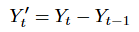
In an ARIMA model, the time series being modeled must be stationary to obtain meaningful predictions. Stationarity is induced by differencing (integration), which refers to the calculation of the difference between adjacent observations, see in (4).
An ARIMA model is a combination of an AR model, an MA model and differencing (integration). If ᴓ = 0 and Ɵ = 0 and Φ = 0, then the time series is a white noise process expressed as in (5) where c is a constant.

The basic notation to describe a non-seasonal ARIMA model is in (6).
where p = the order of the AR part, d = the degree of non-seasonal differentiation, q = the order of the MA part.

If there is stationarity, the ARIMA model is expressed in (7).

in which P = AR terms for the seasonal component, D = the degree of seasonal differentiation, and Q = MA terms for the seasonal component.
The standard form of the ARIMA model is (8), where ᴓ i is the i th coefficient of the autoregressive part and Ɵ i represents the i th coefficient of the moving average.

The Box-Jenkins methodology is used to adjust the ARIMA model forecast. According to Box et al. 35 ARIMA model development is generally best achieved through a three-stage iterative procedure based on identification, estimation, and diagnostic testing. In identification, the time series are analyzed to determine whether they are stationary, and if not, the differences required for their transformation are established. Graphs are constructed to establish the order of AR and MA, based on the calculations of the autocorrelation function of the time series (ACF) and the partial autocorrelation function (PACF).
In the estimation stage, the ARIMA (p, d, q) model is described and its parameters are calculated. In addition, the Akaike information criterion (AIC) and the Bayesian information criterion (BIC) are used in the search for the best model. In the diagnostic tests, several residual plots of the different estimated models are generated, to evaluate the amplitude and variance, with the ACFs, for the evaluation of the trend to normal, and with the behavior of the p-value of the Ljung-Box test.
Results
4.1. Initial data preparation
The open data to be analyzed were downloaded from the Ecuadorian NTA website in a file with CSV extension. The dataset downloaded in the month of January 2023 contained records from January 2017 to December 2022. For this dataset, each row represents information about a transit crash. The first task that was performed was an inspection for NA or null values, with no such expressions found in the downloaded data.
Usually, the original raw data records are too long and may not contain homogeneous information. Therefore, it is necessary to split the data into shorter segments36. The 139,155 records were filtered using the criteria of parish = "Guayaquil" and area = "Urban", resulting in a total of 27,348 records.
4.2. Descriptive analysis
Once the pre-processing of the downloaded data was carried out, a total of 27,348 records remained, representing the total number of accidents that occurred from 2017 to 2022 in the urban area of the parish under study. During that time, 25,460 injuries and 1,022 fatalities were reported.
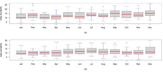
Box plots are used by some authors to better understand the behavior and underlying variation of the data in a time series 37, as well as to identify outliers in the data analyzed. Figure 2 represents a comparison of the box plots for the monthly crash series for the first and last year studied. The presence of outliers was visually detected, which is why the time series must go through a process of leveling them.
Three important indicators stand out as the basis for the quantitative evaluation: the number of accidents, injuries, and deaths on site. Figure 3 shows its behavior within the evaluated time range. Although the number of accidents decreased from 2020 due to the COVID pandemic, the number of deaths has increased.
Evaluating the initial and final year of the data segment under study, it can be reported that in 2017, there were 4,763 transit crashed, 4,403 injured and 139 deceased persons; in 2022 the crashed and injured were less 4,120 and 4,265, but the number of deceased was higher, of 239. Table 1 shows the most significant "probable causes" of accidents, together with the totals and percentages of accidents, and the victims (all injured and deceased persons, occurring at the scene).
Another quantitative variable for characterizing crashes is the time period in which the event occurs. Figure 4 shows the total number of crashes, injuries and deaths for the six years according to the time slot in which the event occurs.
Calculations were also made by the type of crash and type of vehicle, of those injured and killed in the incident. The values and their percentages are shown in Tables 2 and 3, respectively.
Figure 6 shows the different types of crashes and vehicles involved in the accidents, with their percentages of occurrence within the total number of events in the period evaluated.
For each of the events contained in the data, the participating "drivers" who had an age record were identified and the frequency of the number of drivers involved in the accident was processed and grouped by age intervals. It was obtained that the ten age ranges where the largest amount of data under study is concentrated, as the most representative are: from (20 to 25) with 2014, from (25 to 30) with 1868, from (30 to 35) with 1294, from (35 to 40) with 988, from (40 to 45) with 769, from (45 to 50) with 556, from (50 to 55) with 419, from (55 to 60) with 304, from (60 to 65) with 214, from (65 to 70) with 135.
The total frequency value was 9158, which represents 98.8% of the total number of records identified. In the same way, calculations were made to determine the percentage of men and women who were registered as drivers in the crashes, within the defined period of years, with the result that 95% of 16,305 registrations are men and the rest are women.
Predictive analysis
With the descriptive analysis performed, it is confirmed that the most important indicator is the number of crashes, on which the behavior of other variables is descriptively involved; for this reason, its quantitative evaluation and the respective forecast are performed.
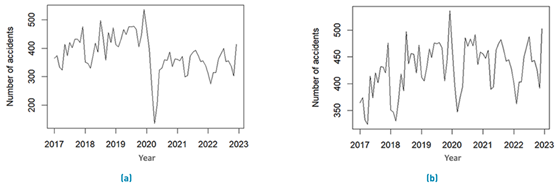
The outliers in the time series may have a moderate to significant impact on the effectiveness of the standard methodology for the analysis of the series. Since outliers were detected during the descriptive analysis of the data, functions from the "tsoutliers" package for R, which is based on the approach described by 38, are used. As a procedure, it decomposes the time series into trend, seasonal and residual elements. Figure 7 presents the plots before and after adjusting the outliers in the crash series.
Stage 1: Identification
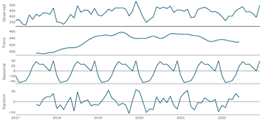
Figure 8 presents the decomposed time series (trend, seasonality, and irregular variation) for its first visual analysis. The trend is calculated with a moving average, the seasonality by averaging the data for each time unit, which in this case is monthly and centering the result, and the irregular variation, which is the observed series minus the trend and seasonality. The trend graph is somewhat flat, but it is not linear, with a slight decrease starting in 2021.
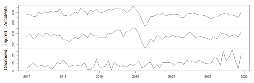
Table 1 Five most significant probable causes of the crashes
| [1] | [2] | [3] | [4] | [5] | [6] | [7] | [8] |
| C09 | Driving a vehicle exceeding the maximum speed limits | 12157 | 44.45 | 10206 | 40.09 | 578 | 56.56 |
| C23 | Not respecting the regulatory traffic signals (stop, yield, red traffic light, etc.) | 5249 | 19.19 | 5977 | 23.48 | 107 | 10.47 |
| C19 | Make sudden or improper lane changes | 2839 | 10.38 | 2894 | 11.37 | 60 | 5.87 |
| C06 | Driving under the influence of alcohol, narcotic or psychotropic substances and/or medication | 2361 | 8.63 | 2167 | 8.51 | 56 | 5.48 |
| C12 | Failure to keep the minimum lateral safety distance between vehicles | 1567 | 5.73 | 1083 | 4.25 | 51 | 4.99 |
Note [1] cause code [2] probable cause [3] total accidents [4] percentage of accidents [5] total injured [6] percentage of injured [7] total fatalities [8] percentage of fatalities
Table 2 Number of injured and deceased by accident type
| Type of crash | Injured | Percentage injured | Deceased | Percentage of deceased |
|---|---|---|---|---|
| Windings | 320 | 1.26 | 54 | 5.28 |
| Run Over | 5272 | 20.71 | 312 | 30.53 |
| Passenger Falls | 506 | 1.99 | 16 | 1.57 |
| Front Crash | 659 | 2.59 | 33 | 3.23 |
| Side Crash | 9833 | 38.62 | 182 | 17.81 |
| Rear Crash | 2146 | 8.43 | 61 | 5.97 |
| Collision | 584 | 2.29 | 1 | 0.10 |
| Crashes | 1493 | 5.86 | 85 | 8.32 |
| Other | 54 | 0.21 | 3 | 0.29 |
| Lane Loss | 994 | 3.90 | 60 | 5.87 |
| Loss Of Track | 2158 | 8.48 | 151 | 14.77 |
| Frictions | 1199 | 4.71 | 48 | 4.70 |
| Overturns | 242 | 0.95 | 16 | 1.57 |

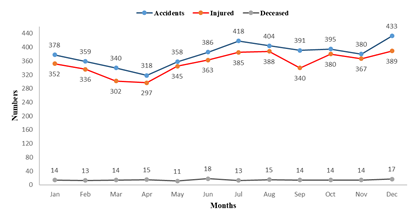
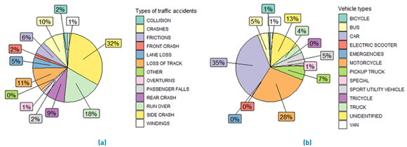
Figure 6 Percentages of accidents from period 2017 to 2022: (a) Types of traffic accidents; (b) Vehicle types
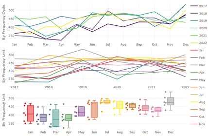
Figure 9 shows three different ways of evaluating the seasonality of the crash series. It can be seen that the seasonal pattern is not similar from year to year. There are fluctuations that indicate there is no seasonality. A new graph was generated by eliminating the growth of the series (trend), but since there is no clarity in the graph, it was not possible to determine a clear seasonality. According to the box plot, the incidence of crashes is high in the month of December.
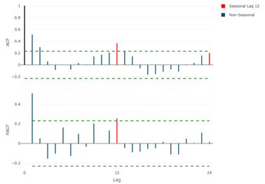
To check whether the time series is stationary, the Dickey-Fuller test is applied using the “adf.test” function, obtaining a p-value equal to 0.04942, which is slightly less than 0.05; therefore, there is a possibility that the null hypothesis is not fulfilled, so the series is probably stationary, and would not require differentiation. Figure 10 shows the ACF and PACF plots with the original series.
Table 3 Number of injuries and deceased by type of vehicle
| Type of vehicle | Injured | Percentage injured | Deceased | Percentage of deceased |
|---|---|---|---|---|
| Car | 7503 | 29.47 | 155 | 15.17 |
| Bicycle | 235 | 0.92 | 10 | 0.98 |
| Bus | 1318 | 5.18 | 84 | 8.22 |
| Truck | 741 | 2.91 | 70 | 6.85 |
| Pickup Truck | 1439 | 5.65 | 50 | 4.89 |
| Emergencies | 5 | 0.02 | 0 | 0.00 |
| Special | 201 | 0.79 | 30 | 2.94 |
| Van | 275 | 1.08 | 4 | 0.39 |
| Motorcycle | 9177 | 36.04 | 419 | 41.00 |
| Unidentified | 3477 | 13.66 | 174 | 17.03 |
| Electric Scooter | 7 | 0.03 | 0 | 0.00 |
| Tricycle | 82 | 0.32 | 1 | 0.10 |
| Sport Utility Vehicle | 1000 | 3.93 | 25 | 2.45 |
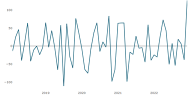
The order of ordinary and seasonal integration (d and D) was verified. The functions “ndiffs” and “nsdiffs” were used, which calculate the numbers of ordinary and seasonal differentiations needed for the series to be stationary. Giving a value of d=1 and D=0. Figure 11 shows the differenced series.
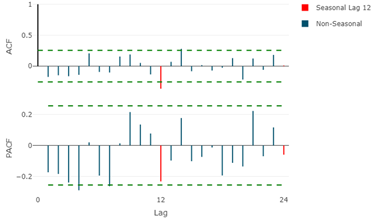
When finding a value d=1, i.e., I, the ACF and PACF plots of the differenced series have to be generated to estimate the possible ARMA(p,q) orders, see Figure 12.
With the presented graph, an ARIMA(1,1,1) was proposed, but seeing that the crash series with the Dickey-Fuller test suggests that the series is stationary, an ARIMA(1,0,3) was also proposed. One of the automated algorithms in R allows the identification of an ARIMA model from the time series. In the "forecast" package, the "auto.arima" function is located, which generates a model resulting from the minimization of the information criteria. When executing the referred function, an ARIMA(0,1,3)(0,0,2) (12, also known as SARIMA (Seasonal Autoregressive Integrated Moving Average Model), which generalizes to all ARIMA models and supports a seasonal component, is proposed as the model of the series.
Stage 2: Estimation
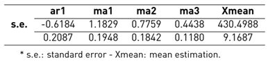
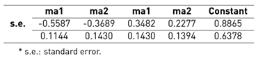
The proposed models created manually from the ACF and PACF graphs are applied, in addition to the model generated by the "auto.arima" function of the "forecast" package; for this purpose, the "sarima" function of the "astsa" package of R was used, which allows fitting an ARIMA(p,d,q) model, see Tables 4, 5 and 6. In addition, this function directly calculates the AIC and BIC values required for evaluation.
One of the most widely used tools for model selection is the information criteria. It allows choosing the model with the best score through comparisons of quantitative scores39.
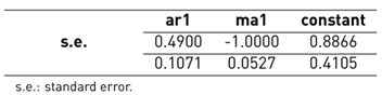
In both the AIC and BIC index, it is established that as the complexity of the model increases, its value increases, and as the probability increases, the value of BIC decreases, i.e., the lower the value of AIC, the better the model fits2. AIC works successfully unless the time dimension is extremely small40. Some studies have pointed out that the overall predictive performance of AIC is better than BIC on some types of problems, while BIC allows better selection of the correct model, such as those evaluated by Chakrabarti & Ghosh 41 and Cavanaugh & Neath42. Table 7 presents the results of the calculated indices of the three models posed.
Stage 3: Diagnostic testing
Box et al. 35 point out that it is necessary to perform tests to verify that the selected model fits the data correctly. It is necessary to verify that the model correctly approximates the original series by checking the residuals, which should behave like white noise, i.e., each autocorrelation should be close to zero. Another criterion to be added in the evaluation is the Ljung-Box test, where if the p-value > 0.05, it means that the residuals of the evaluated model are independent and not autocorrelated. Finally, through the Normal Q-Q plot of the residuals, an approximately normal distribution of the residuals should be shown, to consider that the model is adequate.
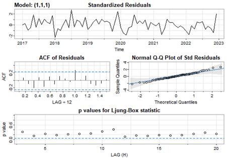
Figure 13 shows four residual plots of the ARIMA(1,1,1) model. In the first one, we can visualize a series of residuals where its amplitude and variance are moderate. The second one, which is the ACF of the residuals, shows a single significant value. The third is a Q-Q (difference diagnosis) graph that shows the approximation of the residuals to the normal distribution. The last graph shows for each delay the p-values of the Ljung-Box test, which allows us to know if the residuals are correlated, being above the margin, and having a p-valuve = 0.1029. It indicates that they are not correlated.
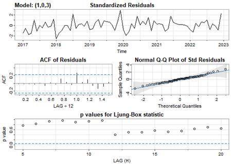
The ARIMA(1,0,3) model with its four residual plots is in Figure 14, with a similar representation to the previous one, with lower significances in the ACF of the residuals, and a p-value = 0.5063 from the Ljung-Box test, also suggests that this is an acceptable model.
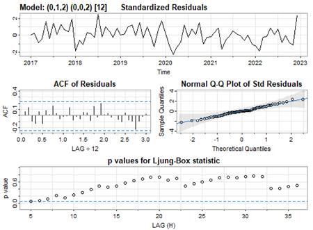
The four graphs of the ARIMA(0,1,2)(0,0,2) (12 model shown in Figure 15, have a representation that highlights the fact that in the ACF of the residuals that do not present a significant value and the calculated p-value of the Ljung-Box test was 0.5245 when evaluating each p-value in the referred graph, it is visualized that they are above the margin, except for the first two that are above it.
Stage 4: Forecast
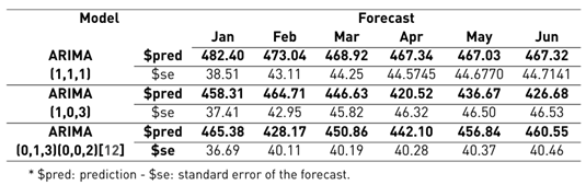
Crash time series forecasts are created based on the three identified models. The 6-month forecast after the end of the analyzed data is performed with the "sarima.for" function of the "astsa" package. Table 8 summarizes the calculated forecast results.
Discussion
This study was conducted with data downloaded from the NTA Ecuador website, corresponding to the months of January 2017 to December 2022. A total of 27,348 records were selected, belonging only to the urban area of Guayaquil parish, due to the difference between the road network and the rural area; this amount represents the number of transit crashes in the referred period. It should be noted that no missing data were identified in the fields of the records evaluated.
The descriptive analysis began with the recognition of the total number of injured and deceased in the period evaluated, which was 25,460 and 1,022, respectively. The behavior of the number of crashes, injuries and deaths was evidenced with a timeline graph, a significant decrease for the year 2020, due to road mobility restrictions imposed globally by COVID, altering the results of the study 19. During the most intense moments of the pandemic, a number decrease was observed, although these were still relatively high and continue to increase 7.

Despite the implementation of various preventive measures, traffic crashes continue to increase 1. This is partly due to the unpredictability and low probability of these events, which makes it difficult to accurately predict their frequency 43.
It is important to note that multiple variables interact to influence the characteristics and frequencies of traffic crashes, generally categorized into human, vehicle, and environmental factors 15. These include the psychomotor status of drivers, vehicle conditions, and the road and weather environment7.
Other factors contributing to variability in the study of traffic crashes include the implementation of stricter speed laws and penalties44, as well as changes in policies that encourage the use of public transport and carpooling24. In addition, regulations by traffic enforcement agencies, such as mandatory technical and mechanical inspections at enforcement centers45, and the use of advanced technologies to monitor risky traffic behaviors in real time20, also play an important role.
Vehicular growth also contributes to the increase in traffic crashes and their negative consequences. In summary, the complexity of these factors requires constant review and evaluation of the road safety situation in each location2.
Box plots were used to visualize the behavior of the claims for the initial (2017) and final (2022) years of the series under study. By observing the amplitude of the boxes and the location of the medians, it can be noted that the series have little stability in the two time periods evaluated both in median and variance. In both cases, there is a significant increase in the number of claims for the month of December, due to the increase in the mobility of the population due to the intense economic activity of the season.
The study reveals that the probable cause of crashes that significantly exceeds any other is "Driving a vehicle exceeding the maximum speed limits" covering 44.45% of the total number of crashes and causing more than half of the total number of fatalities (56.56%). The time slots with the highest number of crashes are in the morning, from 7H00 to 8H59 and in the afternoon, from 15H00 to 16H59; however, the time slots with the highest number of fatalities are at night, from 19H00 to 19H59, and in the early morning from 5H00 to 5H59.
The months with the highest number of traffic transit crashes recorded were December, July, August, and October, respectively, coinciding with patriotic, religious, and cultural festivities in the city. The "side collision" is the main type of crash that occurs, with 32% of the total, followed far behind by "hit-and-run" with 18%. When analyzing the vehicular part, the "automobile" and the "motorcycle" are the most involved in crashes, with a higher percentage, 35% and 28%, respectively. Although the "automobile" is the vehicle most involved in crashes, it is when a "motorcycle" is involved in the crash that the highest number of fatalities is reported, with 41% of the total, making it a high-risk vehicle in the event of a crash.
It appears that 13% of the vehicles involved in the crashes were not identified, and this category contains the second-highest percentage of fatalities, with 17%. This tentatively demonstrates that, once a transit crash occurs, the vehicle involved flees the scene and its participation in the crash cannot be included.
Drivers between 20 and 25 years of age were involved in the majority of crashes in the period analyzed, with 21.70% of the total; very close behind are drivers between 25 and 30 years of age, with 20.10%. When evaluating the percentage of male and female drivers, it is noted that only 60% of crashes in which it was recorded whether the driver was male or female, and of these, 95% were male.
As with any other type of study, it is clear that as much and diverse information as can be obtained and recorded on the phenomena to be analyzed is needed. In addition, subsets of data often show variability that can be considered outliers, due to probable misreporting, where the question remains as to whether or not they should be considered "outliers". For example, in the descriptive analysis of the present study, we found the fact that, when assessing the ages of the drivers in the incidents, one was visualized to be in the age range of 5 to 10 years, and another between 90 and 95 years.
For the reasons described above, the predictive analysis started with the outlier adjustment in the claim’s series, with the "tso" functionality of the "tsoutliers" package for the R programming language. Subsequently, the three stages of the Box-Jenkins methodology were developed to adjust the ARIMA model and build the forecast.
In the identification stage, the time series of claims was decomposed into trend, seasonality, and irregular variation graphs. It was observed that there is no trend; there is only a slight downward trend starting in 2021. A graph was created to evaluate seasonality in three different ways, but it was not possible to clearly visualize seasonality. Only the box plot shows the increase in claims in the month of December, which confirms what was observed in the descriptive study.
The Dickey-Fuller test was used and a p-value of 0.04942 was obtained, which is lower than the 5% significance level (0.05) that is regularly adopted in most analyses, concluding that there is a possibility that the series is stationary and no differentiation would be required; however, since the p-value is so close to 0.05, the evaluation of the model with a differentiation was derived.
When evaluating the order of ordinary and seasonal integration, required to convert the series to stationary, the results indicate that it should be ordinarily differenced once and there should be no differencing for seasonality. Upon differencing, the respective ACF and PACF plots were generated and the ARIMA(1,1,1) model was constructed, i.e. first-order autoregressive (1), first-order integrated(1), with first-order moving average (1).
Seeing that the Dickey-Fuller test described above indicates that the series is stationary, i.e., it did not require differentiation, the ACF and PACF plots of the original series were evaluated, and an autoregressive ARIMA of first order (1), without integration (0), and with moving average of first order (3), i.e., an ARIMA(1,0,3) model, was also proposed.
The execution of the “auto.arima” function of the R language was also considered, which resulted in an ARIMA(0,1,3)(0,0,2) (12, i.e., without autoregression, integrated first order, third order moving average: in the seasonal part, the second order moving average, with a frequency of 12 (monthly). For the estimation stage, the proposed models were applied through the "sarima" function of the "astsa" package of R, which allows fitting an ARIMA(p,d,q) model and even considers the seasonality of the series; it also calculates the AIC and BIC values.
It should be noted that although the "auto. arima" uses a variation of the Hynd-man-Khandakar algorithm 46, where the model values are chosen by minimizing the AICc (corrected AIC) after differencing the data, and presented ARIMA(0,1,3)(0,0,2) (12, as the best model, when reviewing the AIC and BIC indices, they were superior, that is, ARIMA(1,1,1) and ARIMA(1,0,3) are considered the best models.
For the diagnostic tests, we proceeded to check the residuals, with autocorrelation close to zero, and verify that the model approximates the original series. After the tests, it can be concluded that the three models built are acceptable, but the ARIMA(1,0,3) shows slightly better results in the tests. Finally, forecasts were made for the subsequent 6 months of the claims series for the three models defined with the "sarima.for" function of R. As expected, the predicted values are different, with the ARIMA(0,1,3)(0,0,2) (12 model having the lowest forecast standard error value.
Conclusions
Prior to the results of the statistical analysis performed, in compliance with the objective of this study, a literature review was conducted in the Scopus and WoS databases, which demonstrates the interest in the scientific and academic environment to direct their studies in different areas related to transit crashes and the use of time series. An annual growth was evidenced, from 2013 to 2022, in the number of publications, of 15% in Scopus and 26% in WoS. In addition, it can be seen that many of the identified authors propose prediction solutions through ARIMA models.
The results of this research are divided into two sections, which show the past, with a prognosis for the future, of transit crashes in the urban sector of the city of Guayaquil, Ecuador. The first section provides a characterization of the occurrence of transit crashes through a descriptive analysis of the data collected by the highest traffic authorities of Ecuador, and the second section demonstrates the applicability of ARIMA models in the prediction of traffic incidents.
Regarding the descriptive analysis, it can be pointed out that from January 2017 to December 2022, there were 27,348 crashes, and even though the annual number is variable, with a small decrease, it can be assured that the number of fatalities is increasing. In 2022, a total of 239 fatalities were reported, being the highest number recorded in the 6 years evaluated. Due to the outliers found during the descriptive analysis, the data went through an outlier adjustment that has the "tsoutliers" package for R.
The series went through the Box-Jenkins stages to adjust the ARIMA model, first with a decomposition of the series, in which it is visualized that it has no trend; the graphs created do not allow seeing if there is stationarity, but when applying the Dickey-Fuller test the p-value was 0.04942, which means that there is a probability that the series is stationary; however, when evaluating the order of ordinary and seasonal integration, it is indicated that the series should go through a differentiation.
Finally, after evaluating the ACF and PACF graphs, with and without differencing, two models were created; the first one was fitted to an integrated autoregressive and moving average model, both of first order, ARIMA(1,1,1). The second model was a first-order autoregressive with third-order moving averages. A third model was generated with the "auto.arima" function, which was an integrated third-order moving average model with second-order moving average stationarity, with a monthly frequency, ARIMA(0,1,3)(0,0,2) (12. The ARIMA models adjusted for the claim’s series have, in general, similar performances according to the calculation of the AIC and BIC values.
In view of the above, it is proposed to carry out new studies with data provided by the NTA of Ecuador, adding other elements of descriptive analysis and considering the development of other forecasting models to allow comparisons with what has already been developed and their successes. It is recommended that in future studies, the proposed analyses be applied to data from other cities in Latin American countries with similar characteristics to the one studied. All this will make it possible to confirm whether the current results are consistent or whether others are emerging, so that the authorities can promote prevention policies and strategies.

