Inglés (pdf)
 Articulo en XML
 Referencias del artículo
 Enviar articulo por email
 Citado por SciELO
  Citado por Google
  Similares en
SciELO
Similares en
SciELO  Similares en Google
 Permalink
INTRODUCTION
Following the studies of Niskanen (1978), economic literature received different tests of Buchanan and Wagner's hypothesis. Said hypothesis states that public deficit increases expenditure as it reduces the tax price perceived by current tax-payers of public services, thus increasing demand for these services.
Numerous tests of this hypothesis have been conducted for different countries: Niskanen (1978) studied the relationship for USA, Khan (1988) for Pakistan, Craigwell (1991) for small open economies of Barbados, Tridimas (1992) and Asworth (1995) used data from the United Kingdom, Provopoulos (1982), Hondroyiannis and Papa petrou (2001) and Christopoulos and Tsionas (2003) worked with data for Greece, Courakis, Roque-Moura, and Tridimas (1993) for Greece and Portugal, and Yay (2009) studied data for Turkey. As for Spain, this test has been carried out by Raymond and Gonzalez-Páramo (1988) and Jaén (1999). In general terms, the results of the above studies favour the Buchanan- Wagner hypothesis.
In the case of the present study, we analyze a reduced model of the determi nants of public spending growth from a demand side perspective. The model is based on the B-W hypothesis but incorporates several other variables considered, both theoretically and empirically, as determinants of public spending growth. This extension of the work allowed us to analyze the possible of validation of Wagner's Law and the Baumol disparity hypothesis, which are normally formulated in bivari ant models. The formulation of two different equations confirmed the influence of deficit on public spending growth but produced different conclusions in the cases of income, relative prices and population.
In this essay we apply the methodology of unit root and co-integration in time series to make this contrast. On the one hand, this approach allows the elimination of possible problems of spurious regressions that can appear when variables are expressed in levels. On the other hand, it also makes it possible to formulate an er ror correction mechanism associated with co-integration vector, which provides the dynamic of a short run model. The study period considered in Spanish economics1 was 1958-2014 -a period which saw many economic and social changes in the country. To take said changes into consideration, we allow multiple structural breaks in the unit-root and cointegration testing procedures of the series considered.
We obtain two conclusions:
a) In the first equation, we obtain that deficit increases government spending. The coefficient estimated for the income elasticity is positive with a value very close to the unit, which indicates, in line with Wagner's Law, that a rise in income in creases government spending. In the case of relative prices, the value obtained is positive, contradicting the Baumol production disparity hypothesis. Finally, the fact that the population coefficient value is less than 1 suggests economies of scale in public spending as population increases.
b) As regards the second equation, the results obtained are slightly different. The elasticity of public spending is approximately equal to 1, which confirms the B-W hypothesis. Moreover, the income has an elasticity less than 1, which means Wagner's Law is not accepted. Finally, the Baumol disparity hypothesis is validated as it predicts that the relative prices coefficient is negative.
The remainder of this study is divided into five sections. The first section details the information available on expenditure and public deficit evolution during the 1958-2014 period. In the second, we formulate the model, and in the third, we conduct the empirical test using data from the Spanish economy. Finally, in the fourth, a summary is provided which is then followed by corresponding conclusions.
1. PUBLIC EXPENDITURE AND DEFICIT
Recently, Spanish public expenditure has experienced sharp growth in both current prices as well as real prices, and GDP percentages and absolute values.
During the 1958-2014 period, which is being studied in this work, three distinct phases can be identified according to their nature with respect to public expenditure in Spain. The first phase spans from 1958 to 1975, a time in which public expenditure, in real prices, was less than 25% of GDP2. Public spending in the Spanish economy in the first part of this period was very low.
State intervention in the economy was carried out through regulation, which came in the form of laws and statutes. In the 1960's, industrialisation helped increase public expenditure. In true Wagner fashion, economic development went hand in hand with an increase in population, urbanisation, housing, education, health and redistribution of revenue.
During the second period, between 1976 and 1985, a rapid expansion of public spending took place in Spain3. These expenditures increased from 23,19% of GDP to 42,5%, in line with countries in the OECD, whose average spending represented 47% of GDP. Scholars concur that the fundamental driving forces behind this growth in public spending during that time were: 1) the transition to the democracy that produced a boom in demand for social rights, which had previously been withheld by the Franco regime, 2) economic crisis forced enterprises to acquire state grants or capital transfer, 3) the persistence of the budget deficit and its new financing ac cording to market conditions, 4) the decentralization of certain spending auspices without yielding any corresponding fiscal responsibility to the Spanish Autonomous Regions. Also during this time, a tremendous increase in unemployment occurred as a result of the economic recession. In order to mitigate the threat of mass layoffs, an initiative was established that offered the possibility of early retirement.
In the third period, between 1986 and 1993, spending grew as a consequence of the socialist government policy for the Welfare State4. National health cover in creased, as did the number of pensioners under the non-tax paying regime and the quantity of their benefits. The rise in pupils in compulsory and vocational education programmes caused education expenditure to increase as well. Similarly, the agree ment with private education institutions, which entitled them to receive state subsi dies, also caused this spending to jump. In this period of consolidation of Spanish Autonomous Communities, a notable increase in expenditure was implemented by the State but this caused a significant deterioration of the budget balance. Towards the end of this period, the absolute necessity to meet the requirements established by the Maastricht Agreement produced a reduction in the deficit when this had just reached its highest value, 5,9% in relation to GDP in 1993.
Between 1994 and 1998 a drastic change took place in the public sector in Spain. The basic reasons for this switch can be found in the need to meet the conditions of both the Maastrich Agreement and the Stability and Growth Pact, in conjunc tion with the fact that this period coincided with the beginnings of the ascending phase of the economic cycle in 1996. Elevated budget deficits (7,3% of GDP in 1994) dropped to 2,6% in 1998, strictly complying with the condition of the Stability Pact (3% of GDP).
The period between 1999 and 2007 represented a period of consolidation of public finances in Spain, which was primarily based on the real estate bubble that made possible the unprecedented growth of the Spanish economy. Given this new economic setting, a balanced budget was achieved in 2001 with public spending at 40% of GDP while a 4% rise in GDP also took place with respect to the previous period (1997-2001).
From 2007 to 2014 an implosion of the Spanish economy occurred; this was sparked by the bursting of the real estate bubble. At first, expansion continued and the Spanish GDP reached the EU 27 average. As of that moment the Spanish economy, caught in the wake of American and European economies and its own internal problems, entered a severe recession from which it began to emerge in 2014 with some positive GDP growth, albeit modest, (0,08%)5 and with elevated budget deficits (3,5% of GDP in 2013 and 2,5% of GDP in 2014).
Even though contemporary Spanish public expenditure is vastly increasing there is a difference with respect to the rest of the OECD European countries. In 1960, the ratio with regards to GDP was 19,8% in Spain whilst in other European Countries it was 19,5%. Out of the total OECD, the average was 26,6%. In less than thirty years the respective ratios were EU (27) 46,1%, EU (15) 50,9%, and OCDE 41,1. Now, 2014, the ratios are E.U. (27) 48,1%, E.U. (15) 49,2%, OCDE 41,2% and Spain 43,6%.
In Graph 1, we observe the evolution of expenditure in percentages of GDP for both current and real prices. Three stages can be quantified. In current prices, in 1958 the expenditure was 12,54% of GDP while in 1974 that percentage was 21,45%.
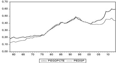
Source: Author's elaboration
Graph 1 Public expenditure/Gross domestic product current and real prices
Over a period of sixteen years, total expenditure increased by 8,89%, thus indicating an annual average increase of 0,56 points.
In 1975, public expenditure was 22,95% of GDP against the 36,9% in 1982, thus revealing a 14% rise, an average annual increase of 1,75 points.
In 1995, it increased to 46,92% of GDP, or 0,72 points on average. The highest value registered, in percentage terms, is seen in 1992 when it reaches 48% of GDP. Due to the need to meet the conditions of the Maastrich Pact, it was not until 1997 when a strong decrease in public spending took place, and in 1998 it had dropped to 42% of GDP. In the years that followed, the need to comply with the Stability and Growth Pact drove the Spanish public sector to its lowest levels since 1980 with public spending in 2006 reaching 38,3% of GDP. The recession in the years to come caused public spending to rise (among other expenditures, there was a conversion of private banking debt into a public sector expenditure), recently placing it at 47,13% of GDP in 2013 and 43,6% of GDP in 2014.
If we consider expenditure as well as GDP in real prices, we can verify that a part of that increase is due to price effect. As many authors, between others Beck (1976, 1981), state government expenditure has a tendency to be overestimated when it is measured at current prices, provided that output growth rate is lower in the public sector due to inherent qualities of public output.
We obtain a better view of that increase if government expenditure is deflated by its own implicit deflator.
At real prices public expenditure in 1958 represented 18,08% of GPD as opposed to 22,31% in 1974, revealing an increase of 5,17% rather than the 8,89% found previ ously. We can attribute 3,72 points of increase, that is to say a 41,8%, to the price effect. In 1975, in real terms, expenditure represented 23,75% of GDP while in 1982 the percentage was 35,52%. Consequently, the increase would be 11,74%, therefore, we can attribute 2,26 points to price effect. In 1995, in real prices, expenditure represented 45,1% of GDP, with an increase of 9,32% in the 82-95 period. Given that in current prices the increase was 10,02%, we can attribute 0,7 points to the price effect. In 1996, in real prices, expenditure represented 43% of GDP, and 43,6% in 2014.
Even though the most significant increase in public deficit occurred after 1975, Fuentes and Barea (1996) believe that in Spanish finance there is a historical trend of public deficit which lies in the strict nature of the fiscal system and the impos sibility of financing vast public expenditures when citizen requirements increase with only a minimum level of tax revenue. Graph 2 shows evolution of public deficit in the period 1958-2014
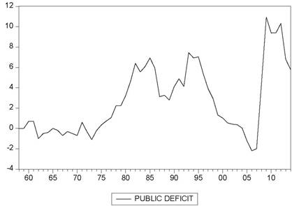
In line with Serrano (1999), there have been three distinct phases in the evolution of deficit in recent years. Increase in deficit had been continuous until 1985. This was caused by a weak government and measures by the opposition of the PSOE who fostered a substantial growth in expenditure and deficit in order to alleviate the economic crisis.
This situation continued in the early years of the socialist government. In the fourth year, the situation improved after Spain's admission into the European Com munity and economic recovery thanks to a favourable period of time in Europe, although the deficit was not completely eliminated.
Between 1990 and 1993 an increase in social expenditure, which was funda mentally brought about by the general strike and the investments in infrastructures for the Olympic Games and Expo'92, in conjunction with its own accrued debt and economic change. In recent years the signing of the Maastricht Agreement meant having to reduce the deficit in order to comply with the entry requirements of the EMU (European Monetary Union). This forced the government to reduce the deficit, which reached a value of 2,9% of GDP in 1998. From 1999 to 2014 there was a period of decline with fiscal surplus from 2005 to 2008. Later, the economic crisis consti tuted a new period of deficit, reaching the maximum in 2012 with 10,32% of GDP.
From a financial point of view, Serrano (1999) and Hernández (1996) identifies two main phases.
Firstly, in matters of finance, the Spanish Central Bank was highly exploited as a resource, and the resources of the financial system were not accessible because of investment ratio. This constituted an inexpensive system, but it interfered with monetary control and also the fight against inflation. This had a negative impact on the efficient distribution of bank credit, mainly due to the goal of maintaining privileged channels of financing for the public sector, thus altering all other prices.
Secondly, since mid-1984, deficit is financed by capital market sources thanks to public debts policy. Essentially, debt is managed by a treasurer with tools to ensure suitable finance of public deficit to permit lower costs. This system has the advantage of not directly affecting monetary policy, however, it produces a lack of finance in the economy as a whole.
2. THE MODEL
Among the various explanations for the increase in public expenditure, the most renown is Buchanan and Wagner's (1977) 7 hypothesis.
According to this hypothesis, budget deficits allow for a higher level of expen diture. Its proposition lies on the premise that public deficits reduce the perceived prices of goods and services provided to the current generation of voters, which, in turn, increases the demand for such social services8.
Niskanen (1978) considers that budget deficit will reduce the perceived prices of federal services by current generations of voters as long as one or a combination of the three conditions is met:
1) Voters are unaware of the future tax liabilities due to current deficits.
2) Voters discount this future tax liability at a higher rate than the interest rate on public debt.
3) Voters have finite lives, and they value the future tax liability during their life more than the liability of subsequent generations.
Once these three conditions are satisfied and there is a negative elasticity of demand of governmental services regarding the perceived tax price, government expenditure will increase.
The model considered in the present study is based on Niskanen (1978), Raymond and Gonzalez-Páramo (1988), Asworth (1995) and Jaén (1999).
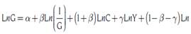
Initially, we take the function of the average taxpayer-voter's demand for govern ment services based on the approximation developed by Borcherding and Deacon (1972) and Bergstrom and Goodman (1973)
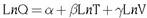 []1
[]1
Q is the amount of government services consumed by the average voter, T is the tax price perceived by the aforementioned average taxpayer-voter and V is the latter's income.
Q is not directly observable, however, the QC product would give us public expenditure per taxpayer with C being unit cost of government services.10
Meanwhile, QCN product gives us total public expenditure with N, the total population. If G = QCN, the result is:
 []2
[]2
T is equal to CF product; C is unit cost of government services and F represents the tax participation in government services paid by the average taxpayer-voter. Likewise, the unit tax participation F is the total fraction of public expenditure and G = QCN paid by taxpayer I. That means F = (I/G)(1/N)11. If total income is considered rather than per capita income Y = VN, the result is
 []3
[]3
Following to Tridimas (1992) and Courakis, Roque-Moura, and Tridimas (1993) we use adequate deflators for the different variables, that is to say, we deflate total government expenditure by its unit cost C; total income (GDP) by its deflator P and we use C/P ratio as the appropriate price variable in the regression equation. The result is
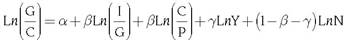 []4
[]4
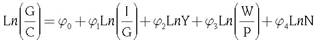
Or, if restrictions set within parameters12are left aside and time consideration is introduced in the model
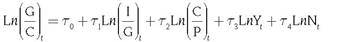 []5
[]5
In this equation τ1 measures the impact of the finance deficit; τ2 and τ3 measure the respective price and income elasticity13 and τ4 is a mixture between the degree of publicity about government spending, the price elasticity and income elasticity and reflects personal preferences.
It is expected that coefficients τ1 and τ2 are negative as opposed to τ3 and τ4, which must be positive.
Similar to the previous model, some authors such as Niskanen (1978), Provo poulos (1982), Craigwell (1991), Hondroyiannis and Papapetrou (2001) Christopoulos and Tsionas (2003), among others14, consider that the unit cost of the bundle of cost services, C, is not measurable but can be a function of the average salary rate in the private sector (Wages) and the number of voters. That is:
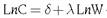 []6
[]6
If the coefficient λ is positive, the productivity growth rate in the public sector is lower than in the private sector. If λ is zero, there is no productivity growth, and if it is negative, productivity in the public sector is greater than in the private sector. The µ coefficient estimates to what extent the government services are "public". If it is equal to zero, the government services are considered to be pure public goods, and if it is equal to one, their cost is proportional to the number of tax-payers/vot ers. And, if it is greater than the unit, there is a crowding-out effect of government services, while if it is negative, there will be economies of scale in the provision of government services.
Starting with Equation (3), and making substitutions with Equation (6) we obtain
 []7
[]7
where φ0 = α+(1+β)δ φ1 = β φ2 = γ φ3 = (1+β)λ φ4 = (1+β)µ+1-β-γ
3. EMPIRICAL TEST OF THE MODEL
If Models (5 and 7) are expressed in levels, there is a risk of producing a spurious regression. In contrast, the model in first differences, despite all likelihood that it obtains stationarity, omits all information in the long-term15. The empirical analysis has to be carried out carefully to verify the nature of the series because if they are not stationary, problems could arise in the estimation of the regression equation coefficients. Valid estimations for the two models require that data be stationary (integrated zero-order) or, if they are not stationary (integrated first-order), they must be cointegrated. More specifically, the first step will be to verify whether the variables are stationary or whether they have one or more unit roots. If they are integrated, an analysis will be made to verify the possible existence of cointegration between them. If they are cointegrated, the relationships or cointegration equations will be estimated. These cointegration equations specify the long-run relationships between the variables. Given the long period of time studied, it is possible to find instances of structural change in the series. For this reason, we allow structural breaks in the series in both the unit root and cointegrating tests. In this view Jaén and Molina (1997, 1999); Asworth (1995); Priesmeier and Koester (2012); Kuckuck, (2014). These structural breaks may be the result of changes in the economy or in the different factors that affect or determine the series utilized. In this situation, if the structural changes are not taken into consideration when the existence of a long-term relationship is investigated, said relationship might not be detected when it does indeed exist.
Following Tridimas (1992); Craigwell (1991); Asworth (1995) and in order to consider the differences between the short and long-term responses to demand the most suitable option is to adopt a vector error correction model for Equation 5.
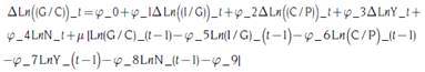 []8
[]8
It avoids the problem of spurious regression because the term
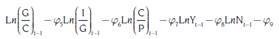 [] 9
[] 9
Is the error correction measurement, that is to say, the long term. That would make the terms in first differences the drifts in the short-term of this long term.
If it is shown that (9) is a cointegration vector, the error correction mechanism gives us the short-term dynamic. In this way, the problems of spurious regression can be avoided and a long-term relationship can be established between expenditure increase and budget deficit. In the same manner, an appropriate methodology can be utilized to carry out the tests in both the short-term and long-term.
Logically, the first step is to establish the integration order of the different time series that specify model variables. This is done through different unit-root tests: Dickey-Fuller (DF or ADF) and Phillips-Perron (PP) among others.
Once the integration order of variables is established, a test can be conducted to determine whether there is a long-term relationship among some or all the variables using the method suggested by Johansen (1991) and Johansen and Juselius (1990, 1992) to test the existence of a cointegration vector. Finally, an additional goal is to find the error correction model corresponding to the cointegration vector mentioned in the previous point.
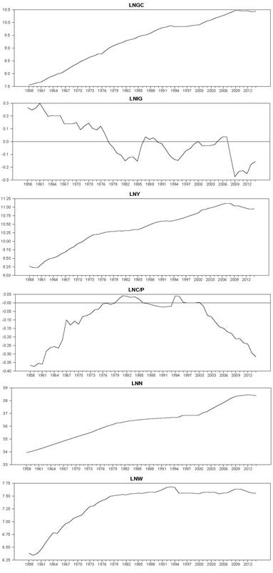
The variables used in the estimation are the following: price index of govern ment expenditures, C is defined as a weighted average of deflators of components of total government expenditure, G is total government expenditure; G/C is total government expenditure deflated by the previous price index; relative price, C/P is ratio of price index of government expenditure divided by implicit GDP deflator; real income Y is measured as GDP to constant price; I is government tax revenue and N is total population17. In the second equation, Ln C/P is replaced by Ln W/P, where W is annual average wage to constant prices.
In Table 1, the data are the results of applying different unit root tests to repre sentative series of variables of the model. It is observed that all the series are order one integrated I(1).
Table 1 Unit root test
| Serie | ADF test | ADFGLS test | PP test | KKPSS test | ERS test | NP test MZa | NP test MZ1 | NP test MSB | NP test MPT | SP test |
| LnG/C | -0,54* | -0,73* | -0,22* | 0,23* | 64,40* | -2,35* | -0,81* | 0,34* | 28,07* | -0,78* |
| Ln I/G | -2,92* | -2,89* | -2,47* | 0,13* | 5,51* | -16,81* | -2,89* | 0,17* | 5,47* | -2,16* |
| Ln Y | -2,26* | -1,90* | -0,43* | 0,18* | 36,65* | -9,49 | -1,94 | 0,20* | 10,54* | -0,98* |
| Ln C/P | -0,42* | -0,41* | 1,15* | 0,23* | 136,98* | -1,23* | -0,49* | 0,39* | 37,55* | -0,89* |
| Ln N | -3,33* | -2,88* | -1,84* | 0,11* | 2,08* | -55,58 | -5,26 | 0,09* | 1,65 | -0,86* |
| Ln W/P | -1,09* | -1,58* | -1,56* | 0,23* | 246,93 | -1,53 | -0,67 | 0,44 | 41,08 | -0,68* |
Source: Author's elaboration
None of the tests reject the null hypothesis of a unit root in time series19. Utiliz ing the graphs20, all the tests are calculated including a constant and a trend in the test equation21: The lags number for ADF was calculated using SIC. The bandwidth for the PP and KPSS test is selected based on Newey-West using Bartlett Kernell.
For ERS and NgP we used Spectral OLS based on SIC. The symbols *, ** and *** indicate significance at 1%, 5%, and 10% using critical values from MacKinnon (1991), KPSS (1992), ERS (1996), NgP (2001) and Schmidt and Phillips (1992).
Table 2 Unit root test for the first differences of the time series
| Serie | ADF test | ADFGLS test | PP test | KKPSS test | ERS test | NP test MZa | NP test MZ1 | NP test MSB | NP test MPT | SP test |
|---|---|---|---|---|---|---|---|---|---|---|
| LnG/C | -4,13* | -4,04* | -4,18* | 0,54* | 1,31* | -19,73* | -3,12* | 0,16* | 1,31 | -4,66* |
| Ln I/G | -5,66* | -5,66* | -5,66* | 0,06 | 0,98* | -25,83* | -3,58* | 0,13* | 0,99 | -5,46* |
| Ln Y | -3,03* | -1,88** | -4,14* | 0,45** | 4,93* | -6,72* | -1,82* | 0,27 | 3,66 | -3,9** |
| Ln C/P | -6,09* | -5,99* | -6,13* | 1,07* | 0,97* | -26,4* | -3,62* | 0,13 | 0,97 | -7,02* |
| Ln N | -1,49 | -1,57 | -2,73** | 0,13 | 4,81* | -6,12* | -1,49* | 0,24* | 4,78 | -3,76** |
| Ln W/P | -4,18 | -3,16 | -4,38 | 0,74 | 2,50 | -14,20 | -2,66 | 0,18 | 1,72 | -3,40** |
Source: Author´s elaboration
There are strong discrepancies among the tests for the first differences in the series. While the first three tests confirm the stationarity of the series in the first four cases, for the Ln N series it is observed that the first difference has a unit root according to the first two tests yet it is stationary according to the rest of the tests.
However, in line with Perron (1989), the standard unit root tests tend to errone ously identify trending stationary processes as stationary in differences and may have very low power, even asymptotically, if changes in regime are ignored. Moreover, during the period studied, there was a great deal of social and political upheaval in Spain, which may have altered the course of public spending and the GDP. Therefore, supposing that the series might have breakpoints, different tests were conducted in order to detect them. Firstly, utilizing the sequential test of Bai-Perron, we obtained up to 3 structural breaks corresponding to the years 1978 (first democratic elections), 1990 (boom and crisis in building sector), and 2005 (beginning of financial and eco nomic crisis). As for the Chow breakpoint test, and using the same breakpoints, it rejects the null hypothesis of non-existence of breakpoints at the points specified.
Given the existence of these breakpoints we conduct unit root tests allowing one or several structural breakpoints at unknown moments in time. The following chart displays the results obtained.
Table 3 Unit root tests considering structural breaks in the data22
| Variable | ZA test | P test | LP test |
|---|---|---|---|
| LnG/C | -3,03 | -3,11 | -3,84 |
| Ln I/G | -4,60 | -4,59 | -4,85 |
| Ln Y | -2,84* | -3,03 | -3,66 |
| Ln C/P | -3,72 | -3,55* | -5,29 |
| Ln N | -4,00 | -3,96 | -4,73 |
| Ln W/P | -3,98* | -4,12* | -4,64 |
Source: Author's elaboration
The tests conducted are Zivot Andrews (1992) unit root test (ZV), Perron (1989) unit root test (P) and Lumsdaine-Papell (1997) Unit root test (LP). All the cases of breakpoints are detected endogeneously by the tests. In the first two cases a maximum of one breakpoint is admitted, while the LP test can detect two or more breakpoints. The ZV test detects breakpoints endogeneously in 1977, 1977, 2005, 2005, 1975 and 1972 for the different variables. In none of the cases does it reject the unit root hypothesis in the variables against the stationary alternative with structural change in both intercept and trend at an unknown date. The P test observes breakpoints in 1976, 1985, 1976, 1996, 1983 for the different variables. The lag selection method belongs to the criteria of Schwartz. It is assumed there is a constant and trend in the data generation process, and that there are breaks in the constant and trend. The critical values are taken from Perron and Vogelsang (1993). The values obtained with alternative specifications confirm the existence of unit roots in all of the variables in every case. The LP test detects breakpoints in 1980 and 1991, 1986 and 1999, 1981 and 2007, 1985 and 2002, 1988 and 1997, and 1971 and 1994 for the different series. In all the cases the statistical test values reveal, in relation to the critical values, that the series have a unit root against the most general alternative hypothesis.
Table 4 Unit root tests for the first differences considering structural breaks in the data
| Variable | ZA test | P test | LP test |
|---|---|---|---|
| LnG/C | -5,39 | -5,40 | -7,57 |
| Ln I/G | -6,64 | -6,63 | -6,81 |
| Ln Y | -5,20 | -7,91 | -7,33 |
| Ln C/P | -5,20 | -7,91 | -7,33 |
| Ln N | -7,91 | -5,20 | -9,20 |
| Ln W/P | -7,18 | -7,92 | -6,88 |
Source: Author's elaboration
We can observe in all the tests that the variables are stationary in first differences.
Both of these preliminary steps are important for ensuring that we employ the correct econometric procedure. The estimation of a cointegrating relationship using Ordinary Least Squares, in general, is biased due to problems of endogeneity with the variables. Consequently, the corresponding t statistics do not follow a normal Student-t distribution, which is why it is not possible to make any kind of inference about its significance. On the other hand, performing a regression on the first dif ference of the variables when there actually exists a long-term relation of balance between them leads to the well-known problem of identifying omitted variables. In fact, what disappears in this type of regression is the error correction term.
Taking into consideration the existence of unit roots in all the model variables, it can be considered that cointegrating relationships do exist among them.
This analysis begins without taking into account the possible structural breaks that may be present among the different variables. In the first model the variables considered were LnG/C, LnI/G, LnY, LnC/P and LnN.
In order to consider the range of cointegration we based our work on the trace statistic and the asymptotic distribution of statistics, and the graph representa tions in cases where we encountered borderline situations. In these cases, we had to consider the behavior of the estimated cointegrating relationships presented in graphic format prior to selecting r. Another diagnostic tool is the use of graphs combined with the number of unit roots of the "matrix companion", which provides information on the pk roots that describe the dynamic properties of the process. This allowed us to see how close the largest unrestricted roots were to the unit circle.
The Johansen-Juselius cointegration test provides us with the following results.
Table 5 Cointegration test without considering breakpoints
| Eigenvalues | Trace Statistic | Critical Value | p-value | |
| r = 0 | 0,55 | 80,13 | 69,61 | 0,000 |
| r = 1 | 0,43 | 43,36 | 47,71 | 0,124 |
| r = 2 | 0,32 | 14,24 | 29,80 | 0.827 |
Source: Author´s elaboration
The r = 0 hypothesis is rejected, which means it has a cointegration vector considering an unrestricted constant in the data.
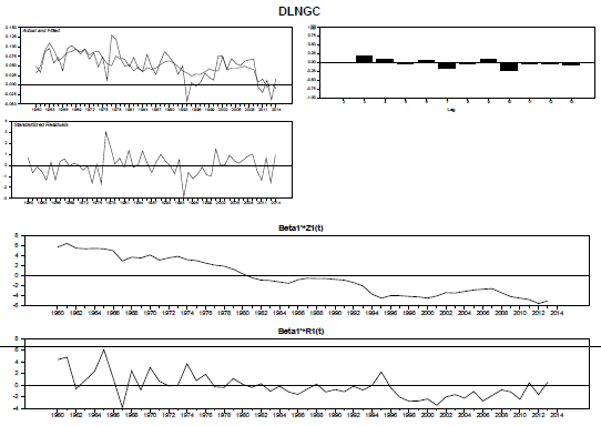
In order to analyze said cointegrating relationship in depth, we conduct various tests. Firstly, we consider the residuals graph.
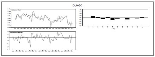
The graphic has four parts: real and adjusted residuals of DLNGC, standardized residuals and histogram of the residuals, the histogram of the density function of the standardized residuals and the density of the normal distribution, as well as the Kolmogorov-Smirnov normality tests23 and the Jarque-Bera test. In the graph, large positive residuals can be observed in 1978, 1990 and 2005, precisely as predicted earlier with the Breush-Pagan test. The analysis of the residuals reveals problems with the normality, likely caused by the structural breaks, while the multivariant LM tests for conditional heterocedasticity are rejected. Finally, the normality test clearly rejects the null hypothesis (existence of normality24).
Secondly, we used the companion matrix where the estimated eigenvalues are the reciprocal values of the roots of the characteristic polynomial A(z); hence, the eigenvalues should be inside the unit disc or equal to 1 under the assumptions of the cointegrated VAR model.
If the process is I(1), the number of roots in the companion matrix is equal to p-r, which is also the number of stochastic tendencies common to the model, which means the roots of A constitute a diagnostic tool to determine the range of ∏ (cointegration matrix). In this case we consider two possibilities: H1 (5) and H1 (2). The former, by construction, possesses all the roots inside the unit circle but, in this case, four of them are very close to 1. As for the latter, three unit roots are significant but it can be observed that the fourth is very close to 1 as well.
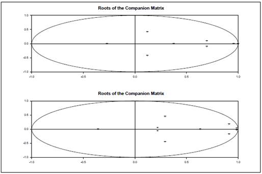
More specifically, in the H1 (2) case the following roots are obtained: 1, 1, 1, 0,956, 0,696; and in the H1 (5): 0,986, 0,986, 0,986, 0,912, 0,632. In the first model (we assume r = 2) we discover three roots equal to 1 but there is a fourth that is very close to 1. In the non-restricted second (r = 5), all the roots are inside the unit circle with four roots very close to 1. In both cases there are four common tendencies, a fact that allows us to state that there is only one cointegrating relationship.
Once the coefficient of the dependent variable is normalized to 1, the cointegra tion vector is [1, -6,87 (-6,40), 2,7 (4,40), -5,30 (-6,45), -2,12 (-6,77)]. We obtained very different values from those that we had expected. If we represent the cointegrating relationship in graph form, we observe that around 1978, 1990 and 2005 there are outliers or breakpoints in the model, precisely as predicted by the Bai-Perron test. These structural breaks must be included in the cointegrating relationship in order to ensure results that agree with the economic reality.
Consequently, we conducted new cointegration tests which included these break points. Given the methodological restrictions of Johansen et al. (2000), we included one or two breakpoints in order to later be able to test whether these breakpoints were the appropriate ones or not.
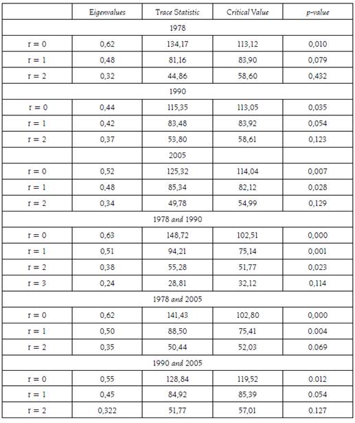
The following table displays the results obtained when considering the break points of 1978, 1999 and 2005, both separately and together.
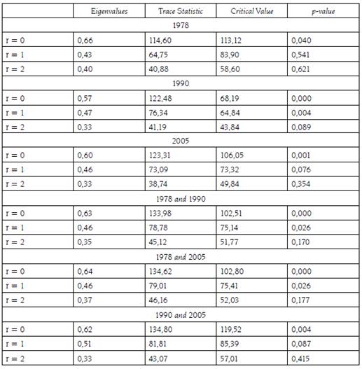
The results in the previous table reveal a cointegrating relationship when con sidering the breakpoint in 1978 and 2005. It also indicates the existence of two cointegration vectors considering the breakpoint in 1990, two cointegration vectors considering 1978 and 1990 and also 1978 and 2005, and one lone cointegration vector considering breakpoints in 1990 and 2005.
Along with the cointegration tests we consider the roots of the companion matrix in each case, as well as the graphs of the cointegrating relationships. The following is a summarized version of the root values of said matrices.
Table 7 Root of the companion matrix for H(2)25
| 1978 | 1990 | 2005 | 1978 and 1990 | |
| Root 1 | 1 | 1 | 1 | 1 |
| Root 2 | 1 | 1 | 1 | 1 |
| Root 3 | 1 | 1 | 1 | 1 |
| Root 4 | 0,986 | 0,972 | 0,943 | 0,963 |
| Root 5 | 0,872 | 0,663 | 0,715 | 0,647 |
| Root 4 | 0,986 | 0,972 | 0,943 | 0,963 |
Source: Author's elaboration
Given the values of the above matrix and the graphs of the cointegrating re lationships, we can conclude, out of all the cases, there is only one cointegrating relationship26, which is summarized in the following table.
Table 8 Cointegration equation in break points27
| LnG/C | LnI/G | LnY | LnC/P | LnN | Break 1 | Break 2 | Cte | |
| 1978 | 1 | -2,24 (-4,65) | 1,60 (2,90) | 1,10 (1,46) | 0,96 (5,20) | 0,06 (1,89) | 16,10 (8,67) | |
| 1990 | 1 | -5,38 (-6,11) | 2,35 (3,12) | 4,64 (5,16) | 1,85 (5,79) | 0,90 (1,06) | 32,78 (7,33) | |
| 2005 | 1 | -5,28 (-7,07) | 2,23 (4,88) | 3,24 (5,32) | 2,05 (7,70) | 0,61 (2,65) | 41,36 (7,77) | |
| 1978 and 2005 | 1 | -2,70 (-6,87) | 0,37 (1,54) | 1,47 (4,68) | 0,94 (6,31) | 0,26 (3,78) | 0,18 (1,41) | 20,90 (6,67) |
| 1978 and 1990 | 1 | -2,34 (-6,47) | 0,29 (0,91) | 1,67 (4,10) | 0,81 (5,69) | 0,28 (4,64) | 0,08 (1,12) | 16,92 (8,46) |
| 1990 and 200528 | 1 | -4,10 (-7,89) | 2,38 (5,33) | 3,27 (5,86) | 1,97 (9,44) | 0,32 (3,05) | 0,51 (3,41) | 37,10 (10,3) |
Source: Author's elaboration
Upon analyzing the above results, we can consider a priori the 1978 and 2005 breakpoints to be significant. The first corresponds to the beginning of the demo cratic era in Spain, while the second marks the start of the current economic crisis.
In view of these considerations, we conduct a reestimation of the cointegration vector taking 1978 and 2005 as breakpoints, along with 1978 and 1990 and, 1990 and 2005. The equations obtained are displayed in the previous table.
We conducted various tests to analyze the suitability of the model. Firstly, dif ferent restrictions were applied to the subsets of the β vectors. We were initially interested in the validation of the structural breaks. To this end, we carried out X2 tests of equality to zero on the coefficients of said breaks. In the case of structural breaks in 1978 and 2005, we found that in the case of the former, the value was χ2(1) = 6,20, with a p-value of 0,013, which clearly rejects the equality to zero of the corresponding coefficient. As for 2005, the value obtained was X2(1) = 1,41, with a p-value of 0,224, which leads us to accept the null hypothesis.
With regard to the structural breaks in 1978 and 1990, the same test provided values of χ2(1) = 0,52, with a p-value of 0,470, which means we cannot reject the null hypothesis of equality to zero for the coefficient corresponding to 1990. In the case of the breakpoint in 1978, the value was χ2(1) = 9,71, with a p-value 0,002, which allows us to reject the null hypothesis of equality to zero for the coefficient corresponding to the breakpoint in 1978.
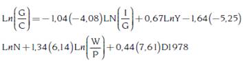
In light of these results, the cointegration vector that should be applied is that corresponding to the 1978 breakpoint, which is displayed in the table above.
Regarding this cointegrating relationship, various hypothesis tests were carried out on its β coefficients. In the tests of equality to zero of the variable coefficients of the cointegrating relationship, we reject the null hypothesis in all cases29. This was not the case in equality to 1 of the LNY coefficient, where we obtained a value of χ2(2) = 4,01, with a p-value of 0,134. Similarly, we accept the null hypothesis in the case of equality to 1 of the population coefficient with a value of χ2(2) = 3,72, with a p-value of 0.155.
Finally, we have conducted weak exogeneity tests on the model variables, reject ing the null hypothesis of exogeneity in all cases.
The results indicate that the deficit has a marked influence on spending growth with an elasticity of 2,24. The LnY coefficient reveals a validation of Wagner's Law during this period30. The coefficient of the price differential would indicate a positive influence on public spending, as well as on the population coefficient, albeit the magnitude of the latter suggests economies of scale in public spending.
Based on the previous cointegrating equation, the corresponding error correction model was formulated and is presented as follows:
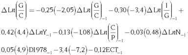 []10
[]10
The error correction model reveals the lack of short-term influence on the indica tive variables of price differential and population.
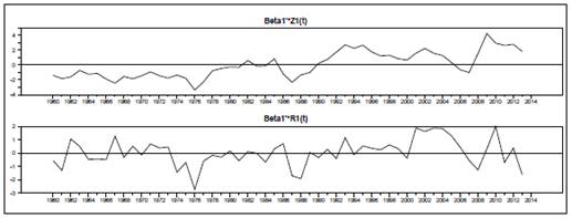
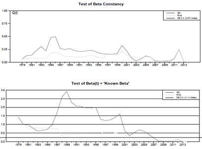
In order to analyze the constancy of the parameters we utilized recursive estima tion methods. The corresponding calculations were carried out in two different ways. Using a basic sampling, we either re-estimated all the parameters in each period (X-form), or we merely re-estimated the long-term estimators of α and β, excluding the short-term dynamic utilizing the parameter estimators in the complete sampling (R1-form).
The first contrast, which was for the constancy of β, revealed the maximum difference between the value of β in the base sampling and the value of β as the sampling size increases. The result indicated that all the values taken throughout the period were in the range below the critical value. The second recursively tests whether any fixed value of β, the estimator of β in the complete sampling, was contained within the expanded space by the estimator of β in the base sampling. Although in method X the behavior was not very suitable (considering that until 2001 the hypothesis was not validated), this was not the case in the second method, in which the hypothesis was validated from 1981.
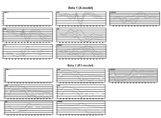
The above graphs show the recursive estimation of the cointegrating equation coefficients using the period 1960-1985 as the base simple. Both graphs reveal that apart from small fluctuations, the estimators of the coefficients of all the model variables are constant. The breakpoint appears again in the form of a peak in the various graphs, followed by a rather steady trajectory thereafter.
We conducted another parallel study, albeit less detailed, utilizing the LnW vari able rather than LnN. Initially, we considered that there were no structural breaks in the data. In those conditions the Johansen-Juselius cointegration test provided the following results:
Table 9 Cointegration test without considering breakpoints
| Eigenvalues | Trace Statistic | Critical Value | p-value | |
|---|---|---|---|---|
| r = 0 | 0,52 | 195,38 | 85,55 | 0,001 |
| r = 1 | 0,38 | 64,58 | 63,66 | 0,041 |
| r = 2 | 0,30 | 38,39 | 42,77 | 0,132 |
Source: Author's elaboration
The hypothesis r = 0 is rejected, which means there is a cointegration vector when considering an unrestricted constant in the data. We have our doubts with regard to the second unit root as both the statistic and the p-value reveal a value close to 0.05. In this case we used the same test methods as in the previous case: residuals, companion matrix and cointegration vector.
In the case of the companion matrix and H(2) we obtained values of 1,1,1,0,939 and 0,686, which provided us with four unit roots and one cointegration vector. The cointegration vector was [1, 4,9 (0,64), -17,29 (-2,01), 4,98 (0,74), 4,5 (0,76)] - a result which is hardly in accordance with the economic reality. Taking into consideration the results obtained for the residuals and cointegration equation, we conducted the same analysis for cointegrating relationships considering the different structural breakpoints. The results are displayed in the following table.
The results in this table indicate a cointegrating relationship when considering the breakpoints in 1978 and 1990 and two cointegrating relationships in 2005.
When two breakpoints are considered, a cointegrating relationship is obtained for 1990 and 2005, two relationships for 1978 and 2005, and up to three relationships for 1978 and 1990.
In order to not overextend the analysis any further we verified that all the cointegrating relationships determined that the hypothesis of equality to zero of the coefficients corresponding to the breakpoints in 1990 and 200532 could not be rejected. Finally, we obtained a cointegration equation corresponding to the breakpoint in 1978:
 []11
[]11
where the equality to zero of the coefficients was rejected in all cases. In the tests of equality to 1, the null was accepted in the case of LnI/G with a value of χ2 (1) = 0,01, with a p-value of 0,925, as well as the equality to 1 of the coefficient LnC/P with χ2(1) = 0,002, with a p-value of 0,925. However, the equality to 1 was rejected for the coefficient LnY with χ2(1) = 9,33 and a p-value of 0.002.
The results reveal an elasticity of the deficit approximately equal to 1, which means the B-W hypothesis is confirmed. Moreover, income has an elasticity of less than 1, meaning that Wagner's Law is accepted. Finally, the Baumol disparity hypothesis would then be confirmed since it predicts that the relative price coef ficient is negative.
Based on the previous cointegration equation, the corresponding error correc tion model was formulated.
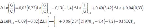 []12
[]12
In parallel to the first model, we also analyzed the constancy of the parameters in the cointegration vector. In this case we limited ourselves to conducting the recursive estimation of the cointegration equation coefficients33.
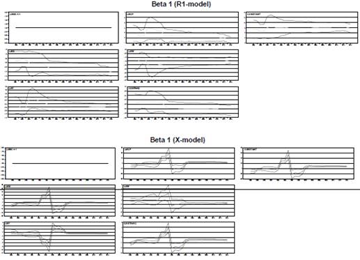
Both graphs show that apart from small fluctuations the estimators of all the model variable coefficients are constant. Another breakpoint appears once again in the form of a peak in the various graphs, followed by a rather steady trajectory thereafter.
4. SUMMARY AND CONCLUSIONS
This study sought to conduct an analysis of public spending growth in Spain based on a reduced model test of the B-W hypothesis. This model also allowed us to analyze the possible validation of one of the versions of Wagner's Law, as well as the Baumol disparity hypothesis.
The present work makes two important contributions to the Spanish literature on this subject. Firstly, it encompasses a significantly longer sampling period than those considered in previous studies, which made it necessary to analyze the major changes that took place in Spain, from both economic and political perspectives. The most notable event was the end of Franco's dictatorship, which gave way to the founding of a democratic government that had to address social demands which, in turn, implied increased public spending. The other two important events that were spurred by economic phenomena were joining the EU and the recent economic crisis. By utilizing techniques like unit roots and cointegration with structural breaks, we came to the conclusion that the only event that significantly affected the trajectory of public spending was the founding of the democratic government. Bearing this in mind, the two alternative equations formulated over the course of the study were estimated.
The coefficients obtained in the first equation allowed us to confirm the validation of the B-W hypothesis, in broad terms. Firstly, precisely as expected, the public deficit coefficient was negative, which implies that a relative increase in tax revenues makes the demand for government spending decrease; or, in other terms, deficit increases government spending. This result is the same as that of Niskanen (1978) Raymond and Gonzalez-Paramo (1988) and Jaén (1999), and it agrees with Buchanan-Wagner's proposition. The coefficient estimated for the income elasticity was positive with a value very close to the unit, which indicates, in line with Wagner's Law, that a rise in income increases government spending. In the case of relative prices, the value obtained was positive, contradicting the Baumol production disparity hypothesis. Finally, the fact that the population coefficient value was less than 1 suggests economies of scale in public spending as population increases.
As regards the second equation, the results obtained were slightly different. The elasticity of public spending is approximately equal to 1, which confirms the B-W hypothesis. Moreover, the income had an elasticity less than 1, which means Wagner's Law is not accepted. Finally, the Baumol disparity hypothesis is validated considering it predicts that the relative prices coefficient is negative.
If we compare the results obtained with the two equations, they are rather dif ferent. On one hand, both cases confirm the B-W hypothesis, but the results for the rest of the variables are quite different. This indicates instability when the variables in the model are changed as merely one modification leads to rather varied results. However, on the other hand, we can observe stability in each model as the param eters obtained in both are constant throughout the various sampling sizes, exactly as shown in the recursive graphs.