Introduction

Worldwide, colorectal cancer (CRC) is the third most common cancer in men and the second most common cancer in women. ¹ In 2012, there were 1.4 million new cases and 694,000 deaths and was the third most common cause of cancer death in the world. ⁽² In Colombia, CCR is the fourth most frequent cause of cancer death in both men and in women. ³ In recent decades, CRC incidence has increased in developed countries unlike the underdeveloped countries where it has remained stable or even decreased. ^1,3,4 Incidence is highest in Australia, New Zealand and Western Europe and lowest in Central Africa and Central and South Asia. ¹ Most CRCs originate from adenomatous polyps of the colon following the polyp-adenocarcinoma sequence. ⁵ Depending on their size, the genome of these lesions may present mutations that start in the APC gene (Adenomatous Polyposis Coli) and then occur in the KRAS and p53 genes. ⁶ The synergism of this mutation determines that small adenomatous polyps and larger polyps become CRC. ⁶ This knowledge is the basis for screening colonoscopy for people 50 years of age or older to reduce CRC mortality by detection and resection of polyps found. ^7,8,9 The intervals between colonoscopic follow-up of patients are determined by the size of the polyps. ^10,11

Nevertheless, current methods for estimating polyp size are inaccurate. Most colonoscopists “measure” the size of polyps by “visual estimation”. This method, even when used by experts, is inaccurate and can overestimate or underestimate true polyp size. ^12,13 Measurements of resected specimens taken in pathology laboratories are smaller than these in-vivo estimates. ^14,15,16,17 When the size is underestimated, very long surveillance intervals can be recommended. These increase the risk of CRC appearing during the interval. ¹⁸ Numerous researchers have looked for methods to measure polyps, including through computerized axial tomography (CAT). ^{13,14,15,16,17,18} Among the various methods, the simplest and most frequently used is to open a biopsy clip near the polyp to compare its size to that of the polyp. Since the size of the open clamp is known to be 5 to 6 mm, it is assumed that this will result in a better estimate. However, the margin of error of this “method” is close to 50%, up or down, even among experts. ¹³ A recent study that used this method found that it correctly determined the size of the polyp in 37% of the cases. The measurement was too large in 34% of cases, and too small in 29%. ¹³ Other methods include use of a calibrated “hood” placed on the tip of the colonoscope. ¹⁹ A study of this method demonstrated that visual estimation is more inaccurate than the hood method, but also found that the hood method is difficult to use. Recently, a complex and sophisticated new method that uses an optical probe and a personal computer has been proposed. It generates a gray scale that allows determination of the size of polyp from the endoscopic image and the distance between the objects. ²⁰ In this investigation, the amplitude of the gray scale was adjusted constantly according to the distance between the tip of the colonoscope and the lesion, since the size of the lesion varies according to the distance. The distance between the objects was calculated according to the amount of laser light reflected from the lesion through an optical probe inserted in the endoscope’s channel. The results of this method led to the conclusion that this system can be used to achieve a more exact determination of polyp size with a conventional endoscope. Nevertheless, cost and difficulty of implementation prevent it from being viable.

Correct measurement of polyp size has two implications: It allows more accurate choice of the size of the loop and polypectomy technique, and improves recommendations for follow-up intervals. If one or more adenomas smaller than 10 mm are found, follow-up colonoscopy should be done every ten years as in screening. However, if there are three to four small polyps, or at least one that measures 10-19 mm, follow up should be done in three years. If there are more than five small polyps, or one that measures 20 mm or more, the next colonoscopy should be in one year. ²¹

Taking into account the need to correctly measure polyps and the absence of a good, widely available, method, we decided to carry out this work with the following objectives.

Overall objective

Our overall objective was to design a method to measure colon polyps during a routine colonoscopy using an algorithm in MATLAB mathematical software.

Materials and methods

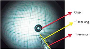
This study was carried out in the Gastroenterology Unit of Clínicas Fundadores in Bogotá, Colombia from August 2014 to August 2016. In the first phase an algorithm was developed in MATLAB software and photos were captured in JPG format with an Olympus Exera II colonoscope. In the second phase, the algorithm was used to estimate sizes of objects which had been previously measured so that the algorithm’s accuracy could be verified. Once correct functioning of the algorithm had been verified, sizes of polyps that had been photographed were estimated with the algorithm. The third phase consisted of estimating the sizes of photographed polyps that had previously been sent to three experts in gastroenterology for visual size estimates. The purpose of this phase was to determine the accuracy of the experts’ visual estimations by comparing them to the algorithm’s measurements. All the photographs used with the MATLAB algorithm were taken with an Olympus Exera II colonoscope in JPG format using the standard protocol. This protocol consists of capturing the images at the distance reached when an Olympus biopsy forceps protruding from the tip of the colonoscope and three rings on the cover of the forceps could be seen. This distance was chosen because we found that it allows an appropriate view of lesions. The biopsy forceps were reusable Olympus steel forceps with a ringed cover. Appropriate positioning was essential and occurred when three of these rings were displayed on the monitor. The standardized distance we chose was 13 mm. Any other device can be used to standardize a distance which can then be entered into the mathematical algorithm thereby maintaining accuracy of measurement. To develop the algorithm, the professional services of an expert MATLAB engineer were contracted. We informed the engineer of our objectives and interest in using this mathematical software containing tools for this type of design (One of us, LOE, is a biomedical engineer).

Patient preparation for colonoscopy was done in split doses in the usual way. ⁹ Briefly, the day before the test, the patient’s diet was normal diet until lunch but afterwards was limited to a liquid diet. At 4:00 PM, the patient started colon cleansing by taking two envelopes of polyethylene glycol with electrolytes (Nulytely®). Each packet was dissolved in one liter of water. Over two hours, the patient ingested a glass of the solution (250 mL) every 15 minutes, consuming one liter per hour for two hours. At 7:00 AM on the day of the exam, the patient repeated this process with two more packets dissolved in water and consumed over two hours. Preparation was finished at 9:00 AM. Two to three hours later, the colonoscopy was performed without sedation and with the patient in left lateral decubitus or supine decubitus. The procedures were executed by an expert colonoscopist, university professor (WOR). The colonoscopies were performed with an Olympus 180 Exera II.

Research phases

Phase 1

This first step in this phase was photographing reference objects with the colonoscope using the JPG format. These objects had known sizes that were supplied by the manufacturer. The reference objects were rubber rings which were made specifically for this investigation by the Discorreas, Mangueras and Empaques S.A. factory in Bogotá. Each ring had its own code and certification printed on the external and internal surfaces. The sizes of the reference objects are shown in Table 1.

Table 1 Rubber rings with known diameters (reference standards) 

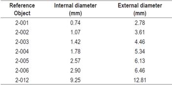
These photos were taken at the same distance from the reference objects as that used to take photos of the polyps (as previously described). Although this distance was not used to make calculations, nor did it influence the development of the algorithm, it was used to standardize captures of images so that each image was taken at the same distance so that they were all comparable and biases were avoided (Figure 1).

Figure 1 Reference pattern with image captured by the colonoscope. 

To estimate sizes of objects, a simple algorithm was designed by expert engineers using functions contained in the MATLAB toolbox.

First, we verified that the algorithm was efficient using different photographs in JPG format. The program was considered to have run properly when the image could be loaded and manipulated with imdistline. The program successively asks the user to enter a number in pixels and then provides a result. The following functions were used in the sequence of operations: “uigetfile”, “imread”, “strcat”, “imshow”, “subplot”, “imdistline”, “Inputdlg”, and “str2double”.

Four variables were created on the basis of these functions. Two of them (A and B) had hypothetical values ​​that were provided by the algorithm for calculation of the value of the fourth variable (D). After this, the value of the third variable (C) is calculated by using the rule of three. Variable A stores a fixed amount of data in pixels, variable B stores a fixed amount of data in millimeters, variable C saves a value that the user enters and variable D performs the rule of three with the data stored in variables A, B and C.

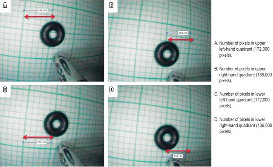
The “msgbox” function shows the result in millimeters that was calculated in the previous process. Once the correct functioning of the algorithm was verified, the number of pixels contained in a certain area, in this case 5 mm, is calculated. To find this value, a photograph in JPG format is placed on a millimeter sheet similar to the one used to measure the rubber ring in Figure 1. A rubber ring with a known size used and then its size was estimated with algorithm that had been established. The four quadrants near the position of the biopsy clip were chosen because this is the position where the polyp is visualized. The “imdistline” function is used to draw a horizontal line on each of the quadrants of the lines of the grid with known size (5 mm) and the pixel value is obtained. The photo we took is shown in Figure 2. The upper and lower right quadrants both measure 172.00 pixels, while the upper and lower left quadrants both measure 139.00 pixels. The values of the grids in pixels differ because the image is convex.

Figure 2 Number of pixels in each quadrant. 

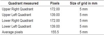
The values ​​obtained in pixels of each of the 5 mm quadrants and the average of these were stored in the algorithm as the reference standard. These values ​​are shown in Table 2.

Table 2 Numbers of pixels in 5 mm quadrants 

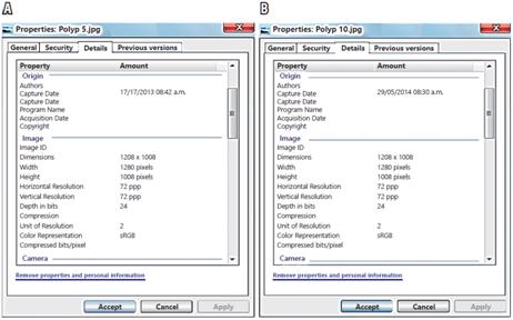
In this first phase, the resolution of the photographs was also verified with respect to the dimensions in pixels and the depth in bits (Shown in Figure 2A and Figure 2B). This verified that all the photos taken in the standardized way contained the information in pixels and depth, regardless of the color of the image and the background color. This contrasts with the method of image segmentation in which the object of study is immersed in the environment and cannot be clearly highlighted by adjusting the number of pixels. With the method chosen in this investigation, the information depends on the distance at which the image is captured during photography since the charge-coupled device (CCD) of the camera of the colonoscope has the property that all the photos taken have the same depth in bits. In this case it was 24 bits, as shown in Figure 3.

Figure 3 Dimensions in pixels and depth in bits of two different photographs. 

We used neither Image processing nor segmentation for these photos, although both can be done in MATLAB because the pixels contained within the object (in this case, the polyps) are similar to or are the same as those in the background of the object (mucosa of the colon).

Phase 2

The final reference pattern of the algorithm, 155.5 pixels contained in a 5 mm grid (see Table 2), allows calculations of the sizes if images entered in JPG format. In this phase, photos of objects with known sizes were used to test the estimates of the algorithm. These objects included photographs of the rubber rings, coins of different denominations, and a skin mole of a volunteer. After loading the image in the algorithm, the “imdistline” function was used and the diameter of the object was measured by drawing a line from one point to another point on the object under study (Figures 4, 5, 6 and 7). The “inputdlg” function opens in a separate window in which the number of pixels previously seen can be entered (Figures 4C, 5C and 6C). Then, the value in millimeters is produced (Figures 4D, 5D and 6D). Other elements with known diameters were also used with the algorithm to establish its accuracy. These included coins of various denominations, open biopsy forceps, a skin mole and colon polyps. These objects are shown in Figures 4, 5 and 6.

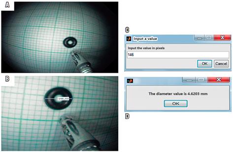
Figure 4 Calculation of the size of a known object in millimeters. A. Photo of a known object (rubber ring), that had already been entered into the algorithm. B. The “imdistline” function is used to measure an object whose size is already known. The line is drawn and the measurement in pixels is obtained. C. The pixel measurement is entered into the algorithm. By clicking “OK”, the measurement is translated into millimeters. 

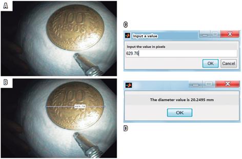
Figure 5 Calculation of the size of a known object in millimeters. A. Object with known size (100 peso coin). B. Measurement in pixels with “imdistline”. C. Window for measurement in pixels. D. Result window showing diameter of the object in millimeters. 

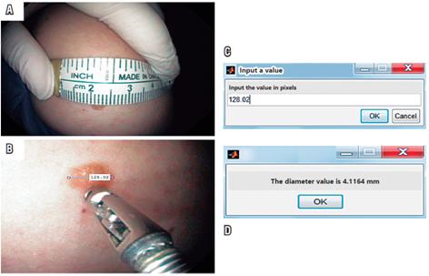
Figure 6 A. Skin lesion with known size B. Measurement in pixels by “imdistline”. C. Window to enter measurement in pixels. D. Result window showing diameter of the object in millimeters. 

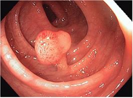
Figure 7 Colon polyp to be measured with the algorithm. Photograph (JGP) taken with colonoscope during a routine colonoscopy. 

In this phase several polyps were also measured using the algorithm. Figure 7 shows one of these, a pedunculated polyp.

Results

The values ​​in pixels and in millimeters that were calculated by the MATLAB algorithm are shown in Figures 5, 6 and 8. Their consolidated values ​​are shown in Table 3. The same table compares the MATLAB algorithm values ​​of each element with each object’s real measurements. It also shows the variations of these two measurements. The signs (+) and (-) indicate that the size supplied by MATLAB is “more than” or less than” than the actual value.

Table 3 Comparisons of objects with known diameters (reference patterns) and algorithm 

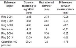
This table shows that the algorithm gives a slightly larger size (one tenth of 1 mm), overestimating sizes by between 0.11 and 0.08 mm, when the object measures less than 5 mm. On the other hand, it underestimates sizes by 0.25 mm when objects are larger than 5 mm. When the object measures 22 mm, the error is 1.76 mm. With these minimal variations, the kappa match is almost perfect.

After verifying the accuracy of the algorithm with objects whose real measurements were known, the size of a polyp found in a colonoscopy was calculated. Its value of 11.09 mm is shown in Figure 8.

Figure 8 Algorithm polyp measurement. 

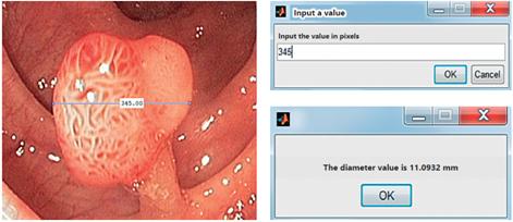
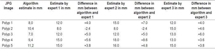
Table 4 shows a comparison of visual measurements by experts and measurements estimated by the algorithm.

The experts estimated that the 7, 8 and 9 mm polyps measured 12, 15 and 18 mm, respectively.

Table 4 Polyp size estimates by expert gastroenterologists compared with MATLAB algorithm estimates 

Discussion

An algorithm designed with MATLAB tools for this study was used to determine the size of real objects with a high degree of agreement with their real measurements. Once adequate performance of the algorithm had been verified, the sizes of colon polyps were estimated. As far as we know, this is the first study that uses MATLAB to estimate the size of colon polyps. With the method developed in this research using an algorithm based on MATLAB mathematical software, measurements are practically exact. For objects smaller than 5 mm, it overestimated sizes by between 0.11 and 0.08 mm. For objects measuring 5 mm, it underestimated the size by 0.25 mm. For objects measuring 22 mm, it underestimated size by 1.76 mm. Overall, the measurement with the algorithm had an inaccuracy of 0.2% to 8% on 22 mm objects. This variation is impressively less than that produced by the experts’ visual estimates which were 50% above or below real measurements. ²¹ Based on this performance, we believe that this algorithm can make it possible to measure colonic polyps before they are removed making its implementation useful in gastroenterology and endoscopy. In addition to the method’s good performance, it is economical and easy to implement. When the visual estimations of experts was compared with the estimations of the algorithm, the experts measurement varied between 50% and 80% above 8 mm polyps with values ​​of 12 mm, 15 mm and 12 mm, respectively. For 7 mm polyps, the experts gave values ​​of 12 mm, 12 mm and 13 mm, respectively, with variations above the real diameter of 50% and 80%. For 11.2 mm polyps, the overestimation was 33% to 40%. If we relied on the measurements of these three experts, patients with polyps that had diameters of 7 and 8 mm would have been scheduled for follow-up colonoscopy within three years since all of the expert estimations were over 10 mm. With these errors of overestimation, costs increase and endoscopy services become congested due to multiplication of unnecessary procedures generated by requests based on erroneously reported sizes over 10 mm. ^10,11 This also represents unjustified costs due to the large number of colonoscopies indicated throughout the country. The results obtained in this investigation allow us to conclude that the accuracy achieved is superior to the other methods now in use.

It is important to emphasize that, although MATLAB has the options of image processing and segmentation, they were not used because of the value of the pixels contained within the polyps. This is similar or equal to the value of the pixels that are in the background of the colonic mucosa which means that a polyp cannot be differentiated enough to isolate it from the values ​​of the environment. A recent study that used the image processing method used a laser to select the polyp from the environment, ²⁰ but this technology is not easy to use due to its complexity and in any case is very expensive.

It is pertinent to note that an important quality indicator of colonoscopy is adherence to the recommendations of guidelines regarding post-polypectomy follow-up colonoscopies. ³¹ Failure to follow guidelines can minimize the impact of a high adenoma detection rate which is considered to be one of the strongest quality indicators of colonoscopy. ³² Follow-up intervals depend on the number of polyps, their histology and their sizes. ^11,31,32 Current European guidelines recommend that the next follow-up colonoscopy should be in ten years when one or two polyps that are smaller than 10 mm are found. On the other hand, if there are three small polyps or at least one polyp that measures 10-20 mm, the colonoscopy should be done in three years. ¹¹ US guidelines make similar recommendations. ²¹ For this reason, measurement of colon polyp size is essential for planning follow-up colonoscopies since they correlate with the risk of CRC. ^5,11,31,32

Conclusions

The algorithm developed with MATLAB provides an excellent approximation of the real size of objects with known measurements. The margins of error were less than 10% in the worst cases. Extrapolating this algorithm to colon polyps makes measurement relatively easy. As in the international studies, measurements by experts overestimated the size of lesions that had been more accurately measured by the algorithm. Theoretically, unnecessary colonoscopies could have been performed based on the expert’s overestimation of polyp size.

Based on the results of this study, we believe that implementation of this method can have a great impact on care of patients with colon polyps and the costs associated. MATLAB mathematical software is relatively easy to use and a simple version can be used for free on the internet. The standard version can be purchased. With the help of an engineer, our system can be implemented easily in any gastroenterology service since it can be downloaded into any computer.

A new method for measuring polyps has been developed.

This original research was designed to solve the universal problem of accurately measuring colon polyps. At this time, we have already begun using our system to measure esophageal and stomach polyps.

Recommendations

Implement this method in endoscopy rooms.

REFERENCES

1. Ferlay J, Shin HR, Bray F, Forman D, Mathers C, Parkin DM. Estimate of worldwide burden of cancer in 2008: GLOBOCAN 2008. Int J Cancer. 2010;127(12):2893-917. doi: 10.1002/ijc.25516. [ Links ]
2. Torre LA, Bray F, Siegel RL, Ferlay J, Lortet-Tieulent J, Jemal A. Global cancer statistics, 2012. CA Cancer J Clin. 2015;65(2):87-108. doi: 10.3322/caac.21262. [ Links ]
3. Piñeros M, Hernández G, Bray F. Increasing mortality rates of common malignancies in Colombia: an emerging problem. Cancer. 2004;101(10):2285-92. [ Links ]
4. Center MM, Jemal A, Ward E. International trends in colorectal cancer incidence rates. Cancer Epidemiol Biomarkers Prev. 2009;18(6):1688-94. doi: 10.1158/1055-9965.EPI-09-0090. [ Links ]
5. MacInnis RJ, English DR, Hopper JL, Haydon AM, Gertig DM, Giles GG. Body size and composition and colon cancer risk in men. Cancer Epidemiol Biomarkers Prev. 2004;13(4):553-9. [ Links ]
6. Vogelstein B, Fearon ER, Hamilton SR, Kern SE, Preisinger AC, Leppert M, et al. Genetic alterations during colorectal-tumor development. N Engl J Med. 1988;319(9):525-32. [ Links ]
7. European Colorectal Cancer Screening Guidelines Working Group, von Karsa L, Patnick J, Segnan N, Atkin W, Halloran S, et al. European guidelines for quality assurance in colorectal cancer screening and diagnosis: overview and introduction to the full supplement publication. Endoscopy. 2013;45(1):51-9. doi: 10.1055/s-0032-1325997. [ Links ]
8. Burges NG, Bahin FF, Bohurque MJ. Colonic polypectomy (with videos). Gastrointest Endosc. 2015;81(4):814-34. doi: 10.1016/j.gie.2014.12.027. [ Links ]
9. Kilgore TW, Abdinoor AA, Szary NM, Schowengerdt SW, Yust JB, Choudhary A, et al. Bowel preparation with split-dose polyethylene glycol before colonoscopy: a meta-analysis of randomized controlled trials. Gastrointest Endosc. 2011;73(6):1240-5. doi: 10.1016/j.gie.2011.02.007. [ Links ]
10. Lieberman DA, Rex DK, Winawer SJ, Giardiello FM, Johnson DA, Levin TR. Guidelines for colonoscopy surveillance after screening and polypectomy: a consensus update by the US Multi-Society Task Force on Colorectal Cancer. Gastroenterology. 2012;143(3):844-57. doi: 10.1053/j.gastro.2012.06.001. [ Links ]
11. Hassan C, Quintero E, Dumonceau JM, Regula J, Brandao C, Chaussade S, et al. Post-polypectomy colonoscopy surveillance: European Society of Gastrointestinal Endoscopy (ESGE) Guideline. Endoscopy. 2013;45(10):842-51. doi: 10.1055/s-0033-1344548. [ Links ]
12. Moug SJ, Vernall N, Saldanha J, McGregor JR, Balsitis M, Diament RH. Endoscopists’ estimation of size should not determine surveillance of colonic polyps. Colon Dis. 2010;12(7):646-50. doi: 10.1111/j.1463-1318.2009.01870.x. [ Links ]
13. Rex DK, Rabinovitz R. Variable interpretation of polyp size by using open forceps by experienced colonoscopists. Gastrointest Endosc. 2014;79(3):402-7. doi: 10.1016/j.gie.2013.08.030. [ Links ]
14. Hofstad B, Vatn M, Larsen S, Osnes M. Reliability of in situ measurements of colorectal polyps. Scand J Gastroenterol. 1992;27(1):59-64. [ Links ]
15. Margulies C, Krevsky B, Catalano MF. How accurate are endoscopic estimates of size? Gastrointest Endosc. 1994;40(2 Pt 1):174-7. [ Links ]
16. Hofstad B, Vatn M, Larsen S, Huitfeldt HS, Osnes M. In situ measurement of colorectal polyps to compare video and fiberoptic endoscopes. Endoscopy. 1994;26(5):461-5. [ Links ]
17. Morales TG, Sampliner RE, Garewal HS, Fennerty MB, Aickin M. The difference in colon polyp size before and after removal. Gastrointest Endosc. 1996;43(1):25-8. [ Links ]
18. Rubio CA, Höög CM, Broström O, Gustavsson J, Karlsson M, Moritz P, et al. Assessing the size of polyp phantoms in tandem colonoscopies. Anticancer Res. 2009;29(5):1539-45. [ Links ]
19. Watanabe T, Kume K, Yoshikawa I, Harada M. Usefulness of a novel calibrated Hood to determine indications for colon polypectomy: visual estimation of polyp size is not accurate. Int J Colorectal Dis. 2015;30(7);933-8. doi: 10.1007/s00384-015-2203-0. [ Links ]
20. Oka K, Seki T, Akatzu T, Wakabayashi T, Inui K, Yoshino J. Clinical study using novel endoscopic system for measuring size of gastrointestinal lesion. World J Gastroenterol. 2014;20(14):4050-8. doi: 10.3748/wjg.v20.i14.4050. [ Links ]
21. Brooks DD, Winawer SJ, Rex DK, Zauber AG, Kahi CJ, Smith RA, et al. Colonoscopy surveillance after polypectomy and colorectal cancer resection. Am Fam Physician. 2008;77(7):995-1002. [ Links ]
22. Anguiano E. ¿Qué es una imagen digital? -Internet-. Fecha de consulta: 27 de enero de 2015. Disponible en: Disponible en: http://arantxa ii.uam.es/~eloy/html/doctorado/doct_9.pdf . [ Links ]
23. Diseño de materiales multimedia. Formato de imagen -Internet-. Fecha de consulta: 27 de enero de 2015. Disponible en: Disponible en: http://www.ite.educacion.es/formacion/materiales/107/cd/imagen/imagen0105.html . [ Links ]
24. masadelanta.com. Definición de qué es un pixel -Internet-. Fecha de consulta: 27 de enero de 2015. Disponible en: Disponible en: http://www.masadelante .com/faqs/pixel . [ Links ]
25. Diseño de materiales multimedia. Web 2.0. Imagen. Conceptos básicos de imagen digital - Internet -. Fecha de consulta: 27 de enero de 2015. Disponible En: Disponible En: http://www.ite.educacion.es/formacion/materiales/107/cd/imagen/pdf/imagen01.pdf . [ Links ]
26. Diccionario de la Real Academia Española. Vigésima Segunda Edición; 2001. [ Links ]
27. MathWorks Blogs -Internet-. Fecha de consulta: 11 de febrero de 2015. Disponible en: Disponible en: http://blogs.mathworks.com/ . [ Links ]
28. MATLAB on StackOverflow -Internet-. Fecha de consulta: 11 de febrero de 2015. Disponible en: Disponible en: http://stackoverflow.com/questions/tagged/matlab . [ Links ]
29. Matlab central -Internet-. Fecha de consulta: 11 de febrero de 2015. Disponible en: Disponible en: http://www.mathworks.com/matlabcentral/ . [ Links ]
30. Moore H. Matlab para ingenieros. México: Editorial Pearso Educación; 2007. [ Links ]
31. Rex DK, Schonfield P, Cohen J, Pike IM, Adler DG, Fennerty MB, et al. Quality indicators for colonoscopy. Gastrointest Endosc. 2015;81(1):31-53. doi: 10.1016/j.gie.2014.07.058. [ Links ]
32. Rees CJ, Bevan R, Zimmermann-Fraedrich K, Rutter MD, Rex D, Dekker E, et al. Expert opinions and scientific evidence for colonoscopy key performance indicators. Gut. 2016;65(12):2045-60. doi: 10.1136/gutjnl-2016-312043. [ Links ]
Received: March 20, 2018; Accepted: April 24, 2018
Este es un artículo publicado en acceso abierto bajo una licencia Creative Commons