http://dx.doi.org/10.15446/agron.colomb.v32n1.39613

¹ External Assessor. Bogota (Colombia).
² Department of Agronomy, Faculty of Agricultural Sciences, Universidad Nacional de Colombia, Bogota (Colombia). gaplazat@unal.edu.co

Received for publication: 23 August, 2013. Accepted for publication: 19 March, 2014.

ABSTRACT

This study aimed to evaluate (at an exploratory level), some of the different conventional sampling designs in a section of a potato crop and in a commercial crop of spinach. Weeds were sampled in a 16 x 48 m section of a potato crop with a set grid of 192 sections. The cover and density of the weeds were registered in squares of from 0.25 to 64 m². The results were used to create a database that allowed for the simulation of different sampling designs: variables and square size. A second sampling was carried out with these results in a spinach crop of 1.16 ha with a set grid of 6 x 6 m cells, evaluating the cover in 4 m² squares. Another database was created with this information, which was used to simulate other sampling designs such as distribution and quantity of sampling squares. According to the obtained results, a good method for approximating the quantity of squares for diverse samples is 10-12 squares (4 m²) for richness per ha and 18 or more squares for abundance per hectare. This square size is optimal since it allows for a sampling of more area without losing sight of low-profile species, with the cover variable best representing the abundance of the weeds.

Key words: vegetables, weed science, crop weed competition, cover, abundance, density.

RESUMEN

Este estudio tuvo como objetivo evaluar (a un nivel exploratorio), algunos de los diferentes diseños de muestreo convencionales en una sección de un cultivo de la papa, y en un cultivo comercial de espinacas. Se realizó un muestreo de malezas en una sección de 16 x 48 m de un cultivo de papa, en red rígida de 192 secciones, en las que se registró la cobertura y la densidad de malezas, en tamaños de cuadro desde 0,25 m², hasta 64 m², con esta información se conformó una base de datos que permitió simular diversos diseños de muestreo como: variables y tamaño de cuadro. Con estos resultados se realizó un segundo muestreo en un cultivo de 1,16 ha de espinaca, en la cual se estableció una red rígida de 6 x 6 m, evaluando la cobertura en cuadros de 4 m². Con esta información se conformó otra base de datos con la cual se simularon otros diseños de muestreo como distribución y cantidad de cuadros muestreados. Según los resultados obtenidos, una buena forma de aproximarse a la cantidad de cuadros para los diversos muestreos es: 10-12 cuadros de 4 m² por ha, para riqueza; 18 o más cuadros para abundancia. Este tamaño de cuadro resulta óptimo, debido a que permite muestrear más área sin perder de vista especies de porte bajo, siendo la cobertura la variable que mejor representa la abundancia de las malezas.

Palabras clave: hortalizas, malherbología, competencia de maleza-cultivo, cobertura, abundancia, densidad.

Introduction

An integrated weed management plan must include a diagnostic stage, which starts with a sampling. In a conventional sense, it is common to use a number of randomly distributed squares in a field, systematic samples such as transects in the shape of an "X", "zigzag" or, in some cases, uniform sampling with a fixed grid and to register variables such as density, cover and frequency of the different encountered weed species (Fuentes, 1986; Gold et al., 1996; Clay and Johnson, 2002).

However, there are situations that must be considered before sampling is started: the selection of the diverse variants of the methodologies depends on the objective of the sampling and the characteristics of the populations (richness and distribution) to be evaluated in each particular agroecosystem (Braun-Blanquet and Oriol de Bolòs, 1979; Matteucci and Colma, 1982; Mostacedo and Fredericksen, 2000).

For Matteucci and Colma (1982), vegetation studies have an objective of: detecting spatial and vertical patterns of the populations, studying population processes that affect them and establishing correlations between the influences of the community and the environment on the distribution of the object population. For Fuentes (1986), the objectives of weed sampling are autoecological studies, production studies and studies on the effects of management practices. Meanwhile, for Leguizamón (2005), they are to detect the presence and abundance of weeds, to obtain information to make management decisions, to construct the "history" of the lot for designing long-term management plans, to detect the appearance of invading species and to provide data for the production of maps that are useful for precision agriculture and supply specific-site management.

Taking these authors' contributions together, weed sampling has two objectives: to reveal the richness and/or the abundance and, in turn, these variables have the objective of providing information for:

•Biodiversity studies: Richness and structure of the communities.
•Short-term management: measurements of abundance for making immediate decisions for the current cycle of the crop.
•Long-term management plans: measurements of richness and abundance for preventative management and evolution of the weed flora.
•Mapping: dynamic spatial studies, site-specific management, patch management.

Currently, in countries with industrial agriculture on a grand scale, different sampling methodologies (e.g., remote perception and continuous sampling) have been evaluated in order to measure their precision in the estimation of abundance and position of the different species (Barroso et al., 2005; LaMastus and Shaw, 2005). However, in the case of Colombia and specifically of the Bogota Plateau where agriculture is non-technical and is carried out in lots of less than 2 ha (DANE, 2001), conventional methodologies for the estimation of the variables of abundance (density, cover, biomass), frequency and distribution (maps) have not been evaluated.

For example, for the number of sampling points, the conventional methodologies for sampling weed populations assume that the populations are distributed homogeneously or randomly (Mostacedo and Fredericksen, 2000; Bautista, 2004) but this is not always the case (Booth et al., 2003) because numerous studies have confirmed that weeds are distributed in patches (González-Andújar and Saavedra, 2003; Heijting et al., 2007; Jurado-Expósitoet al., 2004; Marshall, 1988; Rew and Cousens, 2001).

The distribution of evaluation points in lots should be done with the completely random distribution method when the objective is to evaluate the richness of the species, given the species-area curve; or the minimum area sampling method (Fuentes, 1986). If random (throwing squares), systematic, or uniform sampling schemes are established, the species-area curve stabilizes in a small region of the lot, due to the aggregated distribution of the populations (Rew and Cousens, 2001).

If the objective is the quantification of the populations, the use of layered or slanted sampling distributions is not suitable due to the possibility of over- or underestimating the measured variables because samples may be taken from areas that are overly "representative" (Bautista, 2004), thereby skewing the results. In this case, one must take into account the spatial distribution of the populations: aggregation or "patchiness" (Colbach, et al., 2000); requiring the use of uniform sampling (grids), interpolation and mapping (Rew and Cousens, 2001) or remote sensors (Feyaerts and Van Gool, 2001; Okamoto et al. 2007; Sui et al., 2008).

The size of the sampling unit and the utilized variable mainly depend on the populations that exist in the study area. If it is possible to count individuals in an easy and quick manner, small squares (0.10 to 0.25 m²) can be used to register the density; otherwise, the cover can be registered with medium squares (0.25 to 4.00 m²). If the objective requires higher precision in the estimation of abundance, one can register biomass; and if the populations and areas are large, one can register frequency with methods different from squares or with large squares (>4 m²) (Braun-Blanquet and Oriol de Bolòs, 1979; Fuentes, 1986; Matteucci and Colma, 1982; Mostacedo and Fredericksen, 2000; Bautista, 2004).

For these reasons, the study aimed to evaluate (at an exploratory level), some of the different conventional sampling designs in a section of a potato crop and in a commercial crop of spinach, in order to determine their precision in the estimation of the variables of richness and abundance.

Materials and methods

The present study was carried out in two localities: a potato crop, 4 months after sowing, on the Alcalá farm in the municipality of Cota (Cundinamarca), at an altitude of 2,550 m a.s.l., and with an average temperature of 13°C and a bimodal rainfall regime with 700 mm year^-1. Different square sizes, variables and sampled areas were evaluated. The second area consisted of a crop of spinach, 4 weeks after sowing, located at the Centro Agropecuario Marengo (CAM) in the municipality of Mosquera (Cundinamarca), at an altitude of 2,542 m a.s.l. and with an average temperature of 13°C and a bimodal rainfall regime of 669 mm year^-1. Here, the distribution of the squares and the number of sampling squares were evaluated.

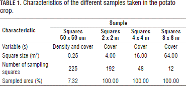
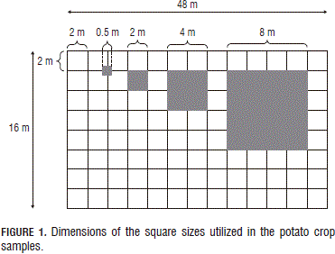
The potato lot was examined and a 16 x 48 m area was selected, which represented the weed conditions of the lot. In this area, a fixed grid of 2 x 2 m cells was constructed. Four samplings were carried out, which are described in Tab. 1 and Fig. 1.

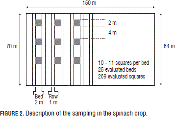
Based on the results of the potato crop, a grid of 6 x 6 m cells was established in the spinach crop in a lot of approximately 1.16 ha. In Fig. 2, one can observe the arrangement of the squares. This type of grid was used because the crops beds were 2 m wide and with 1 m between them, therefore the grid lined up with the spacing of two beds. At each intersection, a 2 x 2 m sample square was used, using the weed cover present in the lot as the measuring variable. A total of 269 squares was used.

Sampling simulation

The information from the sampling points of the fixed grids in the crops was used to produce databases. With the use of coordinates (x, y), evaluated points that correspond to a particular methodology can be extracted.

Evaluation of the number of squares for the estimation of richness. First, the minimum squares technique was simulated, which allows for the detection of the species richness of a community and the minimum number of samples to carry out a subsequent sampling (Fuentes, 1986). One to ten squares were used with ten repetitions for each one in order to obtain the number of registered species with different quantities of squares and to establish the number of squares needed to stabilize the number of species in addition to variance. This process was carried out for both crops.

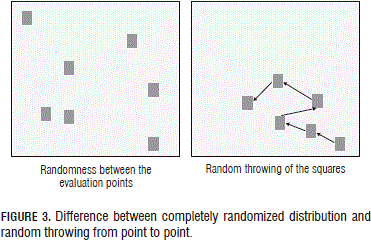
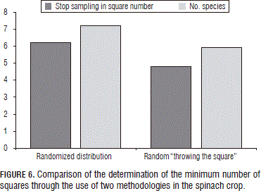
Furthermore, a comparison was carried out in the spinach crop for this technique between a completely randomized distribution, using randomness to select particular data from a group of data, and the random "throwing of the squares" from point to point (Fig. 3).

Evaluation of the square sizes. As can be seen in Tab. 1 and in Fig. 1, the sampling in the potato crop was done with four different square sizes, from 0.25 to 64 m². In this regard, one can observe the differences in the number of registered species and their covers (abundances).

Evaluation of the utilized variable. The density and cover results were compared in the potato crop as variables of abundance in the 0.25 m² squares because, in the larger sized squares, it is impractical to measure this variable by taking the quantity of individuals of the registered species.

Evaluation of the distribution and quantity of squares in the lot in the determination of abundance. In the spinach crop, data were extracted from their respective database to simulate various distributions of the sampling squares in the lot in accordance with the minimum quantity of squares established by the previously-mentioned technique. The simulation contained zigzag, X, random and uniform sampling. In addition, the number of evaluated squares was doubled and tripled.

Results and discussion

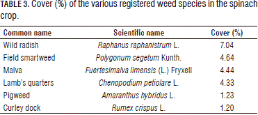
Tables 2 and 3 show the encountered weed species with a mean of abundance, in this case cover.

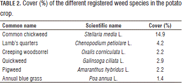
Other species with a mean cover value below 1%: shepherd's purse (Capsella bursa-pastoris L.), common sowthistle (Sonchus oleraceus L.), curly dock (Rumex crispus L.), groundsel (Senecio vulgaris), common cotula (Cotula australis [Sieber ex Spreng.] Hook. F.), ragweeds (Ambrosia sp.), annual nettle (Urtica urens L.), field smartweed (Polygonum segetum Kunth.), corn spurrey (Spergula arvensis L.), morning glory (Ipomoea sp.), common field speedwell (Veronica persica Poir.), pepperweed (Lepidium bipinnatifidum Desv.) and white clover (Trifolium repens L.); for a total of 19 species.

Other species with a percentage of cover below 1%: annual nettle (Urtica urens L.), common cotula (Cotula australis (Sieber ex Spreng.) Hook. F.), knotweed (Polygonum aviculare L.), english canola (Brassica campestris subsp. rapa (L.) Hook. F), sheep sorrel (Rumex acetosella L.) and yellow sorrel (Oxalis corniculata L.); for a total of 12 species.

Evaluation of the number squares and estimation of the richness

Nineteen weeds species were found with the 0.25 m² sampling squares. Meanwhile, with the 4, 16 and 64 m² squares, 17, 16 and 16 species were found, respectively.

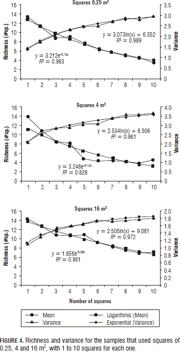
Afterwards, 20 samplings were simulated, randomly taking 1 to 10 squares for each of the square sizes in accordance with the minimum square technique described by Fuentes (1986) and Mostacedo and Fredericksen (2000). The following results were obtained (Fig. 4 and Tab. 4).

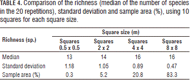
In the evaluation of richness by square sizes, the 0.25 m² squares obtained the highest number of registered species (19) due to the fact that 225 squares were used and 7.32% of the area was sampled (Tab. 1). In addition, smaller squares can reveal in more detail the weed plants that are found in a lot, including the smaller and scarcer plants. On the other hand, with the larger squares, observation was more difficult especially for individuals of the lower layers or of populations of lower abundance, even though the sample area was greater (100%).

However, if the number of observations for all the square sizes is maintained (Tab. 4), the sampled area increases with the size of the squares; and the number of encountered species increases and the standard deviation decreases. But, in the best cases (16 and 64 m² squares), 16 of the 20 total encountered species were registered.

The three square sizes were fitted to models for richness (logarithmic) and for variance (negative exponential) and high R² values (>96%) were obtained (Fig. 4). According to Fuentes (1986), the minimum number of squares is found where the curve stabilizes for more than three consecutive squares. In this case, the curves stabilized after six squares for all the square sizes, obtaining a richness of 12 species.

For the spinach crop (Fig. 5), high R² values were observed in the fitting to the models: logarithmic for richness and negative exponential for variance. Here, the curve presented three consecutive results with six squares; however, the total quantity of species was twelve.

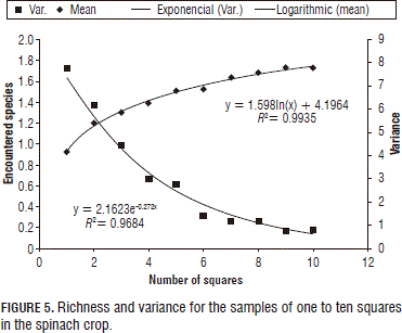
Assuming in this case that finding 80% of the species present is acceptable, according to the adjusted models, the number of squares for registering 80% of the species present can be seen in Tab. 5.

As can be seen in Fig. 6, the randomized distribution method requires more squares to stabilize the species-area curve and so registered more species than the randomly-thrown squares method with a statistically significant difference according to a Tukey test. These differences were due to the fact that, for the thrown squares, the evaluated points were not sufficiently separated to capture other species given the spatial dependence of the variable, which is to say the distribution in patches. Meanwhile, for the evaluation points of the randomized distribution method, the position of the squares did not depend on the spatial position of the other points.

Evaluation of the square sizes

The cover variable was compared in three square sizes (0.25, 4 and 16 m²) for the crop species and two weed species (S. media and C. petiolare) because S. media was the dominant species (14.9%) in the lot, followed by C. petiolare (4.2%), albeit at a far lower rate than S. mediaI, the other weed species had low cover values in the lot.

Table 6 shows that the crop plants had higher cover estimation in the larger square sizes due to their age and profile, rather than the fact that they were the crop, which covered the weeds present in the lot that had smaller sizes than the crop at the sampling time. For the same reason, the estimation of the cover of the weed plants decreased with increases in the square sizes.

Evaluation of the utilized variable

The cover variable was compared to the density variable for the 0.25 m² square sampling for the two previously-mentioned weed species and the crop species.

As can be seen in Tab. 7, there was a relationship between the number of plants and their cover, because it is intrinsic to each species and to the phenological state. However, the plants that dominated the lot were the potato crop and S. media, and C. petiolare was less competitive due to the state it was found in. For this reason and in this particular case, cover was more appropriate as a variable of abundance because it better approximated the true state of the lot. The cover variable, in a qualitative manner, better explained the abundance of the populations. However, certain situations exist where the cover of the community is very high and very low, cases that increase the observational error of the evaluator for the cover of each species. In these cases, it is better to use another variable (e.g., reproductive structure counts) with smaller squares.

Evaluation of the quantity and distribution of the squares in the lot for the determination of abundance

The lowest value for the coefficient of variation was presented by the general sample with 268 evaluation points. However, the coefficient increased when a species with a higher aggregation index was evaluated; with a correlation of 0.9991. This indicates that when a species has a higher degree of aggregation, the sampling will be less reliable in the estimation of the abundance variable for the entire lot (Cottam et al., 1957). As a result, it is vital to find these types of populations and use site-specific management (Wiles, 2005).

For species with a more uniform distribution, the distribution method of the evaluation points is not so important in the estimation of this variable. The quantity of the evaluation points does affect the reliability of the results. This can be seen in Tab. 8 in the upper-left square, which corresponds to the crop species (Cottam et al., 1957).

With an increase in the degree of aggregation, the reliability of the estimation of cover in the zigzag, X and randomized distribution methods depends on the position of the weed patches in the lot and on how many points can be registered; as in the case of U. urens, which was not registered in the randomized distribution, X and zigzag methods that had the lowest quantities of points or the zigzag method with the highest number of points; the zigzag method with a medium quantity of points only registered it in one of the 12 sites.

The grid method with a high quantity of points generally presented low coefficients of variance and a value close to that of the general sample because it guarantees a more uniform sample and a high probability of finding patches of aggregated species.

However, for species with a high or medium degree of aggregation, an abundance value of a lot lacks the reliability needed for any decision-making process.

Conclusions

When estimating the richness of a weed species in a lot, it is preferable to use a large quantity of small squares (<4 m²) because they allow for a more detailed exploration of the lower layers and for finding species that have a low profile or that are scarcer.

For the estimation of richness, the minimum square technique must use the randomized distribution method and not the randomly-thrown method in order to be effective. That is to say, the squares must be randomly dispersed throughout the entire lot and not just thrown or spread out from the starting point of the sampling. This is because weeds have a spatial dependence (aggregation) which makes the species-area curve arrive at its limit quickly, without registering other species.

According to the results, in these cases, a good method of approximating the quantity of squares for diverse samples is: (10-12) 4 m² squares per ha for richness samples and 18 or more squares for abundance.

In general, cover is a variable that is easy to measure, fast and reliable because large squares can be used (>4m²) which allows for the sampling of a larger area. In addition, as observed with C. petiolare in the potato crop, cover estimates the abundance of the weeds better than density because the latter depends on the phenological state of the plants.

For the estimation of abundance variables, the zigzag, X, and randomized samplings depend on luck for obtaining information of the different patches and precision is lower when the populations are more aggregated. For example, U. urens, the species with the highest aggregate index, was not reported in the X and zigzag samplings with low numbers of points. On the other hand, the uniform samples find the principal weed patches. And so, it is better to use systematic and uniform (grids) samplings, working down in the size of the squares in accordance with the characteristics of the lot and the size and profile of the weeds and the crop.

In accordance with the results obtained for the potato crop, 4 m² squares are appropriate for diverse sampling circumstances because smaller squares do not register a sufficient area and can result in numerous empty squares. Very large squares (16 m²) overestimate the abundance value of the dominant population and underestimate the values of the scarce populations.

Using a general value for abundance is not advisable because of the aggregation of the weeds. That is to say, a given value could have a degree of statistical reliability but from the technical point of view that value will be representative for only a fraction of a lot. For example, in the present study, for U. urens, whose average cover was 0.12%, this value was too low to be considered a threat to the crop but there was a 90% patch value at harvest. As a result, in this particular area, this species became more important, highlighting the importance of site-specific or patch-specific management.

Acknowledgements

The authors wish to thank the División de Investigación Sede Bogota of the Universidad Nacional de Colombia for their support through the Project: "Dinámica de las poblaciones de malezas en el cultivo de espinaca (Spinacea oleracea L.), en la Hacienda Marengo, Mosquera-Cundinamarca" code 10952 from the conference on "Apoyo a tesis de programas de posgrado Sede Bogotá - año 2009".

Literature cited

Barroso, J., D. Ruiz, C. Fernandez-Quintanilla, E.S. Leguizamon, P.J. Hernaiz, A. Ribeiro, B. Diaz, B.D. Maxwell, and L.J. Rew. 2005. Comparison of sampling methodologies for site-specific management of Avena sterilis. Weed Res. 45(3), 165-174.         [ Links ]

Bautista Z., F. 2004. Técnicas de muestreo para manejadores de recursos naturales. Universidad Nacional Autónoma de México (UNAM), Mexico DF.         [ Links ]

Booth, B., S. Murphy, and C. Swanton. 2003. Weed ecology in natural and agricultural systems. CAB International, Wallingford, UK.         [ Links ]

Braun-Blanquet, J. and J.L.J. Oriol de Bolòs. 1979. Fitosociología. Bases para el estudio de las comunidades vegetales. H. Blume Ediciones, Madrid.         [ Links ]

Clay, S. and G. Johnson. 2002. Scouting for weeds (on line). Crop Manage. 1(1).         [ Links ]

Colbach, N., F. Dessaint, and F. Forcella. 2000. Evaluating field-scale sampling methods for the estimation of mean plant densities of weeds. Weed Res. 40(5), 411-430.         [ Links ]

Cottam, G., J.T. Curtis, and A.J. Catana. 1957. Some sampling characteristics of a series of aggregated populations. Ecol. 38(4), 610-622.         [ Links ]

Feyaerts, F. and L. Van Gool. 2001. Multi-spectral vision system for weed detection. Pattern Recogn. Lett. 22(6-7), 667-674.         [ Links ]

Fuentes, C.L. 1986. Metodología y técnicas para evaluar las poblaciones de malezas y su efecto en los cultivos. Rev. Comalfi 13, 29-50.         [ Links ]

Gold, H.J., J. Bay, and G.G. Wilkerson. 1996. Scouting for weeds, based on the negative binomial distribution. Weed Sci. 44, 504-510.         [ Links ]

González-Andújar, J.L. and M. Saavedra. 2003. Spatial distribution of annual grass weed populations in winter cereals. Crop Prot. 22(4), 629-633.         [ Links ]

Heijting, S., W. Van der Werf, A. Stein, and M.J. Kropff. 2007. Are weed patches stable in location? Application of an explicitly two-dimensional methodology. Weed Res. 47, 381-395.         [ Links ]

Jurado-Expósito, M., F. Lopez-Granados, J.L. González-Andújar, and L. García-Torres. 2004. Spatial and temporal analysis of Convolvulus arvensis L. populations over four growing seasons. Eur. J. Agron. 21(3), 287-296.         [ Links ]

LaMastus, F.E. and D.R. Shaw. 2005. Comparison of different sampling scales to estimate weed populations in three soybean fields. Precis. Agric. 6(3), 271-280.         [ Links ]

Leguizamón, E.S. 2005. El manejo de malezas en el campo. Rev. Agromensajes 17, 26-29.         [ Links ]

Marshall, E.J.P. 1988. Field-scale estimates of grass weed populations in arable land. Weed Res. 28(3), 191-198.         [ Links ]

Matteucci, S.D. and A. Colma. 1982. Metodología para el estudio de la vegetación. Biology Series No. 22. The General Secretariat of the Organization of American States, Washington DC.         [ Links ]

Mostacedo, B. and T.S. Fredericksen. 2000. Manual de métodos básicos de muestreo y análisis en ecología vegetal. Bolfor, Santa Cruz de la Sierra, Bolivia.         [ Links ]

Okamoto, H., T. Murata, T. Kataoka, and S.I. Hata. 2007. Plant classification for weed detection using hyperspectral imaging with wavelet analysis. Weed Biol. Manage. 7(1), 31-37.         [ Links ]

Rew, L.J. and R.D. Cousens. 2001. Spatial distribution of weeds in arable crops: are current sampling and analytical methods appropriate? Weed Res. 41(1), 1-18.         [ Links ]

Sui, R., J.A. Thomasson, J. Hanks, and J. Wooten. 2008. Ground-based sensing system for weed mapping in cotton. Comput. Electron. Agric. 60(1), 31-38.         [ Links ]

Wiles, L.J. 2005. Sampling to make maps for site-specific weed management. Weed Sci. 53(2), 228-235.         [ Links ]