


 Inglês (pdf)
 Artigo em XML
 Referências do artigo
 Enviar este artigo por email
 Citado por SciELO
  Citado por Google
  Similares em
SciELO
Similares em
SciELO  Similares em Google
 Permalink
Introduction
During the last 40 years, crop systems simulation has evolved from a neophyte science with inadequate computer power into a robust and increasingly accepted science supported by improved software and computing capabilities (Boote et al., 2012). Over the last decade, the most significant demand of cropping system models has aimed to assess climate change impact on agriculture and to evaluate mitigation and adaptation strategies, conducted over different spatial scales and degrees of agricultural systems complexity (Stöckle et al., 2014).
Most crop system models have evolved as elaborations of crop components and soil models focusing on modeling a single point in space over time to explore the of crop responses to soil, management and weather variability (Jones, et al., 2016). Regarding the crop modeling component, they simulate phenology and partitioning, and integrate processes of C, N and water balance from planting to maturity, showing the final yield and production as well as the daily values of crop components over the time to maturity (Boote et al., 2013). This potential yield is related to an adapted cultivar mainly determined by solar radiation, temperature, carbon dioxide, and genetic traits that lead the length of the growing period, light interception by the crop canopy and its conversion to biomass, and the biomass partition to the harvestable organs (Grassini et al., 2015). Under this approach, crop growth is not constrained by factors such as water, nutrients or pests.
While in the developed world the description and testing of single crop models have lost relevance (Stöckle et al., 2014), the development of crop growth models remains as a distant study subject to less developed agricultural productive areas. Di Paola et al. (2015) showed an overview of the crop growth and yield models through the unbalanced situation in which most of the available models have been applied for temperate regions and some references exhibiting examples from Brazil and Mexico. Moreover, the development of such models has been oriented towards staple crops such as cereals, sugar beet and potato.
Tomato is among the most important horticultural crops worldwide. A variety of tomato growth models have been developed in the past (i.e. Soto et al., 2014; Valdés-Gómez et al., 2014; Heuvelink, 1999; Scholberg, et al, 1997; Jones et al., 1991) with different levels of complexity and for different purposes. Tomato crop growth models have been included in decision support systems such as the world-renowned DSSAT (Jones et al., 2003) as well as many others (Massa et al., 2013; Jizhang et al., 2006). Moreover, 3D models of tomato plants have been developed for purposes such as optimizing LED lighting to increase light absorption and crop growth (de Visser et al, 2014).
In Colombia, Cooman (2002) evaluated the feasibility of a protected tomato cropping in the high altitude tropics by locally calibrating the second version of the Tomgro model through controlled experiments in the Bogota plateau. He modified the model by reducing the leaf expansion rate at low temperature and incorporating a direct effect of temperature on the distribution of dry matter between vegetative and generative plant organs. This modified version of the Tomgro model was later applied by Bojacá et al. (2009) to evaluate the variability of greenhouse tomato yield caused by spatial temperature variations.
However, most of Colombian tomatoes are grown throughout the year in several Andean mountain valleys and hills in warmer climates at altitudes below those of the Bogota plateau. Regarding the production context, tomato is a small-scale business represented by clusters of growers cultivating tomato by one of the two established systems: open field or greenhouse production. Under both systems, growers apply suboptimal practices despite the differences on the demand for resources per unit area (Bojacá et al., 2013; 2014).
As process based, crop models closely reflect the behavior of particular crops, the features of Colombian tomato systems demand the development of a locally calibrated growth model. However, this calibration is a highly data-demanding task as well as specific for the available data constraining a broader applicability (Robertson et al, 2013). On the other hand, most calibration experiments are carried out under controlled conditions, which in some cases are not representative of those observed under the natural field conditions (Craufurd et al, 2013).
Thus, the objective of the present work is to propose a simple crop growth tomato model with the ability to simulate different growth habits (open field or greenhouse) calibrated through on-farm trials, which reproduce the growing patterns and management practices applied by local farmers in Colombia. While on-farm calibration entails a series of experimental challenges, it allows the development of a more realistic model reproducing the production management practices applied by growers in the considered zones.
Materials and methods
Model description
The model structure, as presented in Figure 1, is based on earlier crop growth and transpiration models (Gil et al., 2017; Cooman, 2002). The model runs on a daily basis, exception made for the gross photosynthesis and maintenance respiration routines, which run on an hourly basis. All model calculations are done on a per plant basis. At the beginning of the simulation, once the climate (air temperature, relative humidity and global radiation) for the corresponding day is updated, the total dry matter production is simulated followed by its distribution among the above-ground plant organs.
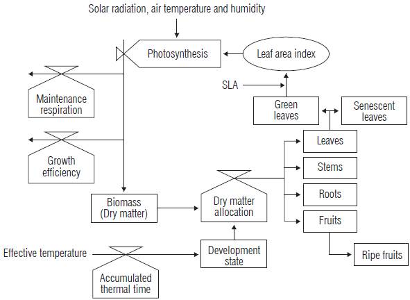
Dry matter production
The amount of dry matter available for growth is calculated at the end of the day as the difference between gross photosynthesis and total respiration. The daily gross photosynthesis results from the integration of the photosynthetic rates calculated on an hourly basis. The photosynthetic rate depends mainly on the photosynthetic active radiation (PAR) absorbed by the canopy, the air temperature and the CO2 concentration, as modeled by Acock et al. (1978). The model considers restrictions on the photosynthetic rate due t o extreme temperatures and vapor pressure deficit. These processes were modeled with the following equations:
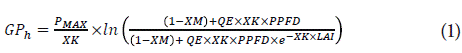


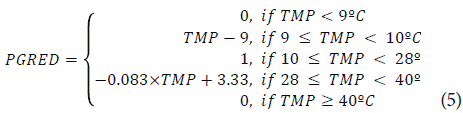
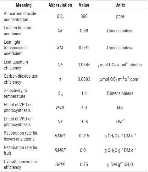
Where GP h is the hourly gross photosyn the sis (g CH2O h-1), P MAX is t he maxi mum leaf photo synthetic rate (μmol CO2 m-2 s-1), XK is the light extinction coefficient, XM is the leaf light transmission coefficient, QE is the leaf quantum efficiency (μmol CO2 μmol -1 photon), PPFD is the photosynthetic photon flux density μmol m-2 s-1), LAI is the leaf area index, Sol Rad is the hourly solar radiation (MJ m-2), τ is the CO2 use efficiency μmol CO2 m-2 s-1 ppm-1), CO2 is the carbon dioxide concentration in air (ppm), PVPD is a function that correct the P MAX for air vapor pressure deficit, CK is a factor used to determine the effect of vapor pressure deficit on photosynthesis (kPa-1), VPD is the air vapor pressure deficit (kPa), VPDL is a factor used to determine trie effect of vapor pressure deficit on photosynthesis (kPa), PGRED is a function that correct the P MAX for sub optimal temperatures and TMP is the hourly mean temperature (°C).
At the end of each day hourly gross photosynthesis is integrated, and the results is transformed into the amount of carbohydrates synthesized by the plantat the currentday, following this formula:

where GP d is daily gross photosynthe sis (g CH2O d-1), GP h is hourly gross photosynthesis (g CH2O h-1) and PLM2 is the plant density (plants/m2).
The total respiration is represented by the maintenance respiration and the growth efficiency. Daily maintenance respiration is calculated as a fraction of the accumulated dry matter in stems, active leaves and growing fruits at a reference temperature of 20°C. Afterward s, the maintenance respiration is corrected for temperature using a Q10 value. Next we present the equations that describe this module.

where M RES is the maintenance respiration per day (g CH2O d-1), TMP avg is the daily average temperature (°C), RMRL is a respiration coefficient for stem and lea<estissues (g CH2O g-1 DM d-1), DMl is the dry matter in leaves (g DM), DMs is the dry matter in stems (g IDM), RMRF is a respiration coefficient for growing fruits (g CH2O g- 1 DM <-1 ) and DMf is the dry matter in fruits (g DM) .
Based on the above, the daily biomass production per plant is calculated using th e following expression:

Where DMp is the total dry matter produced at day (g DM d-1), GP d is the dailygross photosynthesis (g CH2O d-1), M RES is the maintenance respiration per day (g CH2O d-1) and GREF is a growth efficiency coefficient (g DM g-1 CH2O).
Dry matter distribution
We considered the orga ns in th e model as single un its (i.e. big leaf model approach),meaning no dry matter distribution occurred among cohorts or sympodial units. The dry matter fabricated each day is allocked to the plant organs thro ugh thermal time (TT, °Cd) dependent functions. Each function describes the proportion (on a scale from 0 to 1) of the daily dry matter assigned to the considered organ . The base temperature at which plant growth starts was set at 10°C (Valdés-Gómez et al, 2014). A fixed fraction (9%) of the dry matter produced was allocated to the roots. The equations describing dry matter distribution are:


Where DMp is the total dry matter produced at day (g DM d-1), DM¡ is the daily dry matter allocated to leaves (g DM d-1), DMf is the daily dry matter allocated to fruits (g DM d-1), DM S is the daily dry matter allocated to stems (g DM d-1), DM r is the daily dry matter allocated to roots (g DM d-1), ATT is accumulated thermal time (°Cd) and a i , b i , c i and d i are the parameters that must be fitted for each function,and the sub index i represents the corresponding plant organ (leaves and fruits).
Once leaf se nescence starts, the fraction of dry matter distributed to these leaves was estimated as a function of the ATT. When the harvest begins, we applied the same approach for the ripe fruits. Th e daily leaf area was calculated as the total dry matter correspo nding to the active 1 e a fs multiplied by the specific leaf area (SLA). The proportion of senescent leaves was calculated in the following; way for open field tomatoes:
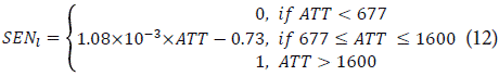
While for tomatoes under greenhouse it was calculated as follows:

where SEN ¡ is the rate of senesce s for leaves, ATT is accumulated thermal time (°Cd), ase„, b sen , and c sen , are the parameters to be fitted. On the other hand, ripe fruits ready to be harvested were сalculated with the following function:
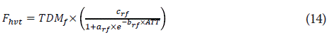
where F hvt is the dry matter of ripe fruits (g DM), TDM f is the accumuleted drymatter in fruits throughout the crop cycle (g DM), ATT repre sents the accumulated thermal time (°Cd) and a rf b rf and c rf are the parameters that must be fitted. The leaf airea (LA) per plant was calculated based on the DM allocated to leaves and the SLA according to the following expression:


where LA is the plant leaf area (m2 plant-1), TDM gl is total dry matter belonging to photosynthetically active leaves (g DM), SLA is the specific leaf area (m2 g-1) estimated as 0.019 and 0.021 for greenhouse and open field tomatoes, respectively, TDM l is total dry matter allocated in leaves (g DM) and SEN l is the rate of senesces for leaves. Finally, the ATT was calculated as follows:

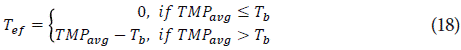
where ATT is accumulated thermal ti me (°Cd), nd is the number of days of the growing cycle, T ef is the daily effective temperature (°C), TMP avg is the daily average temperature (°C) and T b is the base temperature (10°C). The values of the parametefs i ncluded in the previous models equations are shown in Tab. 1; while the values of the fitted parameters values (ai, b i ,, c i , d i ) for the equations 9, 10, 13 and 14 are shown in the Results section.
Field experiments
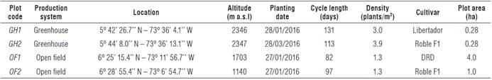
The experimental work was conducted during 2016 in four commercial tomato production plots, with two of them planted under open field and the other two under greenhouse conditions. On each case, the crops were planted and managed according to the commercial practices regularly applied by growers under each production system. The crops were planted in two of the most representative tomato production areas of Colombia. The Alto Ricaurte province, located in the department of Boyaca, is one of the major greenhouse tomato production areas in Colombia, while the Guanenta province situated in the department of Santander is an important production area for open field vegetables including tomato. Tab. 2 describes the general characteristics of the experiments carried out to calibrate the proposed crop growth model. Next, we present a general description of the management practices applied in the experimental fields for both production systems.
TABLE 2 General characteristics of the on-farm experiments used to calibrate the tomato crop growth model.
The protected experiments were carried out under plastic naturally ventilated greenhouses with wooden structure. Plants were grown on a single stem of indeterminate length by periodically removing side shoots. Plants were tutored following the high wire system and no fruit pruning was done whatsoever. After harvest began, the leaves located under the harvested truss were removed since these no longer contributed to the plant growth and were more susceptible to be infected by fungal diseases. Nutrients were delivered through a fertigation system along with the irrigation water.
For the open field experiments, determinate growth cultivars grew freely without doing any leaf or fruit pruning, hanging the shoots to an elevated wire. Solid fertilization was done throughout the cropping cycle with amounts and timing defined by each grower. Fertilization for each location was based on soil analysis results, and the nutrients demanded by the plant to achieve potential yields. Under greenhouse, the fertilization of macronutrients was defined based on the following reference extractions: 10, 6.7 and 20 g/plant for nitrogen (as total nitrogen), phosphorus (as P2O5) and potassium (as K2O), respectively. For the open field plots, the reference values were 12.3, 6.9 and 19.3 g/plant of nitrogen (as total nitrogen), phosphorus (as P2O5) and potassium (as K2O), respectively. These values were obtained from the literature (Besford and Maw, 1974; Hernández et al., 2009; Atherton and Rudich, 2012) and adjusted based on previous trials conducted. The fertilization was divided into two periods taking into account the plant development stage. The establishment stage was defined from the sowing until the appearance of the first truss while the second one corresponded to the fruits development.
We took into account that the first stage has a shorter duration and that during most of the tomato cycle, the plants alternate between vegetative and generative growth. The fertilization fragmentation was done as follows: 30% of nitrogen and phosphorus, and 20% of potassium during the establishment and the rest during the fruit development stage. In the open field, the fertilizers used were ammonium nitrate, diammonium phosphate and potassium chloride, while under greenhouse the sources were calcium nitrate, monoammonium phosphate, and potassium sulfate. In the open field plots, we applied the fertilizers manually on a fortnightly basis, while under greenhouse we did it through the fertigation system three times a week. Under both systems, pest management was entirely based on chemically synthetized pesticides and with a spraying schedule defined according to the grower's criteria.
Data collection
The model calibration data were collected through a series of destructive measurements carried out for each experimental plot. Starting at transplanting time and on a fortnightly basis, the aerial part of three plants from each experimental plot was removed. Under all conditions, the sampled plants were surrounded by edge plants. Afterwards, the plants were divided into its organs and weighted after being oven dried at 70°C for at least 72 h. The leaf weight included the weight of the blades and all petioles.
Once fruit harvest and leaf pruning began, the amount of biomass removed from the plant was registered, and a sample was taken to determine its dry matter content. The grower defined the frequency and amount of biomass harvested or removed according to his criteria. the leaf area was determined by taking digital pictures of all the active leaves present at the moment of the destructive measurement. From the digital pictures, the number of pixels representing the leaves was extracted, including a reference object of a known area. To discriminate the image pixels as leaves, a reference object included into a prediction tree algorithm was used. All pictures were taken at the same height through a fixed mount tripod. The corresponding leaf area was estimated through the relation between the number of pixels of the reference object and the number of pixels corresponding to the leaf surface. This image processing step was carried out with the R statistical software (R Core Team, 2015). All the data collected from fruit harvest, leaf pruning and leaf area was later then integrated on a per plant basis.
The length of the data collection calibration was a function of the grower's decision to continue with his crop. Therefore, the number of destructive measurements was variable particularly to each experimental plot. Regularly, greenhouse growers are able to extend the cropping cycle for a longer period than those of the open field system. For the greenhouse plots we were able to carry out ten and nine destructive measurements for GH1 and GH2, respectively, while for the open field plots seven and eight destructive measurements for OF1 and OF2 were respectively performed. In all cases, the destructive measurements were carried out until the end of the cropping cycle, ensuring that the complete plant cycle was characterized through these measurements. Tab. 1 includes the duration of the crop cycle for each experiment.
As global radiation, air temperature, relative humidity and wind speed are input variables for the model, Data was collected by placing the required sensors within the experimental plots. The hourly weather was recorded using a Vantage Pro2 Weather System (Davis Instruments, Hayward, CA, USA) for each of the open field experimental plots. For the greenhouse plots, Two copper-constantan thermocouples were installed and linked to a datalogger (Cox-Tracer Junior, Escort DLS, Edison, NJ, USA) to register dry and wet bulb temperatures. Through the psychrometric relationship between these two temperatures the air relative humidity was derived. Thermocouples were placed inside a ventilated white capsule to avoid altered readings due to the sun direct radiation. The global radiation within the greenhouses was measured throughout the measurement period with a pyranometer (Model LI200RX, Campbell Scientific, Inc., Logan, UT, USA) placed at 2.5 m above the ground. A weather station was deployed (Model Vantage Pro2, Davis Instruments, Hayward, CA, USA) outside the greenhouses, registering the external hourly climate.
Dry matter partitioning calibration
The calibration of the proposed model was focused on the dry matter partitioning among organs while it is considered as a key process to define the overall growth and development of the plant. For this purpose, on each tomato system, individual models to the fractions were fitted defining the amount of daily dry matter allocated at the leaves (Equation 9) and fruits (Equation 10) as a function of TT. The parameters for each model were estimated through the Nelder-Mead algorithm for a derivative-free optimization (Kelley, 1999) implemented in the dfoptim package (Varadhan, 2016) of the R statistical computing software (R Core Team, 2015). The same procedure was followed for the models that defined the fractions of senescent leaves (Equation 13) and ripe fruits (Equation 14).
A fixed fraction of 9% was allocated to the dry matter of the roots (Gil et al., 2017). The fraction of dry matter allocated to the stems was calculated as the remaining fraction after d iscounting those allocated to fruits, leaves and roots.
The statistical analysis comparing the observed field data and the simulated values included the following statistical criteria: Bias (g DM /plant), root mean s quare error (RMSE, g DM/plant), and model efficiency (EF, dimensionless). These goodness-of-fit measures are defined according to the following; equations:


Where N is the total number of observations, D ¡ is the difference between the measured value (Y i ) and the observed one (Ŷ) for the ith observation. Bias quantifies the average difference between measured and simulated values, with the best fit indicated when the Bias index is closer to zero. The RMSE is in the same units of the original variable and is a measure commonly used to check the agreement between measured and simulated results. EF is the most widely used distance measure including upper and lower bounds (Wallach, 2006). A model with an EF equal to one indicates a perfect fit between observed and predicted values. A full description of these goodness-of-fit measures can be found in Wallach (2006).
Results and discussion
Experimental climate conditions
The climate conditions under which the calibration experiments were carried out are summarized in Tab. 3. The climate conditions for the greenhouse experiments were similar since both greenhouses were located near to each other in the same municipality. However, by being planted in different dates resulted in some climate differences, especially those related to radiation levels. The global radiation level experienced by plants of the GH1 experiment was higher than the one observed for the GH2 experiment.
TABLE 3 Daily averages of the climate variables registered during the cali bration experiments carried out under greenhouse and open field conditions
| Plot code | Temperature (°C) | Global radiation (W m2) | Relative humidity (%) |
|---|---|---|---|
| GH1 | 17.4 | 132.4 | 75.5 |
| GH2 | 17.9 | 113.3 | 76.4 |
| OF1 | 20.6 | 123.9 | 82.6 |
| OF2 | 24.0 | 220.3 | 76.9 |
As the open field experiments were located at a lower altitude, these plants grew at higher temperatures with averages above 20°C. The climate of the OF2 experiment showed the highest temperature and radiation levels as compared to the other three experiments. The lower radiation levels of the other experiments are explained due to the plastic covering in the case of the greenhouse experiments and by the geographical location of the OF1 experiment.
This open field experiment was located on top of a mountain with a permanent cloud cover, observed throughout the data collection period.
The temperatures registered in the open field experiments were more suitable for tomato cropping than those of the greenhouse experiments. Despite the use of plastic coverings, the average temperature of the night hours (18:00-5:00) were 15.4 and 14.8°C for the GH1 and GH2 experiments, respectively, while for the OF1 and OF2 experiments were 18.5 and 21.3°C, respectively. During the day hours (6:00-17:00), the GH1 experiment showed an average temperature of 19.4°C while the temperature within the GH2 experiment was warmer with an average of 21°C. Higher daily temperatures were observed for the open field experiments with averages of 22.8 and 26.7°C for OF1 and OF2, respectively.
Dry matter distribution calibration
The dry matter allocation to the plant organs is a process linked to the total dry matter accumulation of the plant. Since the daily amount of assimilates produced by the photosynthesis process is a function of the climate conditions but also of the available leaf area, then the dry matter fraction allocated to the leaves defines the daily dry matter produced by the plant. Therefore, with the calibration of the dry matter distributed to leaves and fruits, we simultaneously calibrated the total dry matter plant accumulation. The fitted parameters of the functions defining the fractions of daily dry matter allocated to leaves (Equation 9), fruits (Equation 10), senescent leaves (Equation 13) and ripe fruits (Equation 14) as a function of TT are presented in Tab. 4.
TABLE 4 Fitted parameters for the dry matter allocation in leaves (DM,) and fruits (DM,), leaves senescence rate (SEN) and ripening fruit rate (F hvt ).
| Open field | Greenhouse | |||||||
|---|---|---|---|---|---|---|---|---|
| Fraction | a | b | c | d | a | b | c | d |
| Dm, | 0.044 | -0.005 | 0.547 | 0.251 | 0.006 | -0.012 | 0.377 | 0.301 |
| Dm, | 51.34 | 0.006 | 0.521 | - | 136.23 | 0.012 | 0.543 | - |
| SEN, | - | - | - | - | 3,239.37 | 0.011 | 0.735 | - |
| F hvt | 10,830 | 0.009 | 0.668 | - | 1,000.00 | 0.009 | 0.668 | - |
As the dry matter distribution fractions were calibrated as a function of TT, next we present the cumulated TT of the four experiments. The highest accumulation of TT was achieved by the OF2 experiment with a value of 1,371.5°Cd and followed by GH1 with 972.5°Cd. GH2 and OF1 experiments reached similar TTs of 888.7 and 885.6°Cd, respectively. Since the dry matter distribution fractions are calibrated in function of temperature we remove the time effect, allowing a more general application of these temperature-dependent functions. Therefore, the temperatures under which the plants grew are determinant for their development process rather than the cycle length.
The graphical representation of the dry matter distribution functions to the plant organs is depicted in Figure 2. The initial calibration procedure considered unique dry matter distribution functions for both tomato types. However, the results of this calibration procedure and the lower values of the goodness of fit measures indicated that independent calibration procedures should be followed for each tomato production system.
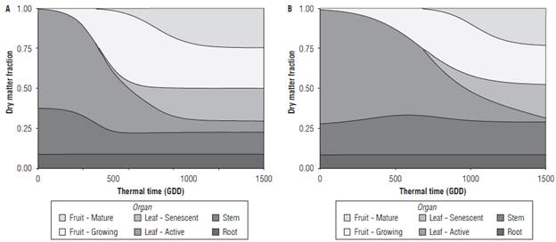
FIGURE 2 (A) Greenhouse and (B) open field tomato dry matter distribution fraction as a function of thermal time for each of the plant organs and its stages.
As stated previously, the fraction allocated to the roots was fixed to 0.09, while for the aboveground organs, the calibration was carried out for the leaves and fruits fractions. After adding up all the fractions, the stem fraction was the one needed to reach the total amount of dry matter produced as a function of TT. The comparison between production systems, exhibit the differences in the dry matter allocation to the plant organs. Under greenhouse conditions, tomatoes showed a higher decline in the dry matter allocated to the leaves and stems as compared to the situation observed for the open field tomatoes. Even under open field conditions, the plant starts allocating a higher proportion of assimilates to the leaves and then, the stem fraction increases and stabilizes to a value of 0.2.
The observed behavior of the organ fractions is defined by the growing habit of each tomato type and the way each production system is handled by the growers. Under open field conditions, tomato cultivars are mostly related to a determinate growth rate and growers do not apply any shoots pruning. Therefore, these plants have a higher stem fraction as compared to the indeterminate single-stem tomatoes planted under greenhouse conditions.
After a longer vegetative growth stage, the photosynthetically active leaves fraction of the open field plants declines to a minimum at the end of the growing cycle. Most of the remaining leaves hanging on the plant belong to the senescent fraction. On the other hand, a higher and constant fraction of active leaves is observed for the greenhouse plants, a situation that is characteristic of their indeterminate growth habit.
The fraction allocated to the fruits in the open field tomatoes showed a gentle slope as compared to the trend observed for the greenhouse conditions. However, at the end of the growth cycle, the fraction of ripe and growing fruits takes over about half of the dry matter produced by the plant. While the same pattern is observed for greenhouse tomatoes, in this case the fruits fraction is stabilized and remains constant at around the 1000°Cd. Under both production systems, it is important to note the fraction of growing fruits that remain on the plant. As the crop is reaching the end of its production cycle, the amount of harvested fruit should be higher than the one remaining in the plant, especially in the case of open field tomatoes. Nevertheless, under the local conditions growers do not properly balance the vegetative and generative growth of the plant nor apply proper pollination and pruning strategies, leading to this kind of results.
Once the dry matter distribution functions for each tomato type were calibrated, they were incorporated into the model. The observed and simulated total dry matter per plant and its allocation to the plant organs is presented in Figure 3. In most cases, the simulated dry matter properly followed the pattern depicted by the observed field data. The observed data also included not only the average of the sampled plants but also the standard deviation as a dispersion measure. Especially for the open field experiments and in particular for the last destructive measurements, there was an important variation in the data collected in the field.
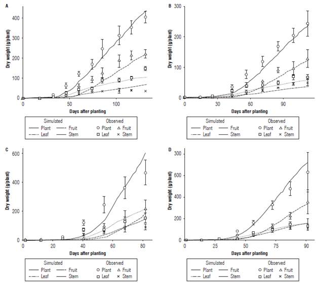
FIGURE 3 Observed and simulated dry matter accumulation and distribution over the plant organs for the calibration experiments carried out under (A, B) greenhouse and (C, D) open field conditions. Vertical bars represent the estimated standard deviation.
Table 5 presents the goodness of fit measures selected to establish the crop growth model performance as compared to the observed field data. As the dry matter allocation fractions to the plant organs were estimated independently to each tomato type, we also present the goodness of fit measures per type of production system. According to the results for the whole plant and for each organ, a better model is considered to fit to the open field condition since values were closer to zero than the obtained ones for greenhouse tomatoes (Tab. 5). In most cases, the Bias results are positive indicating that the model tends to under-predict especially for the fruit dry matter since the higher Bias value was obtained for this organ and for both systems. The under-prediction reported by this index is a common pattern observed in particular for the first measurement dates (Fig. 3). Only the Bias for the total dry matter per plant in the open field condition was negative, indicating an overall over-prediction of the model but the Bias as such was close to zero (Tab. 5).
TABLE 5 Goodness of fit measures of the simulated dry matter per plant and per organ by the calibrated tomato crop growth model.

According to the results, the highest RMSE was obtained for the total dry matter per plant of the open field plants. The RMSE for the other plant organs and also for the results of the greenhouse plants yielded comparable RMSE values. Looking only at the results for the organs, the simulated dry matter allocated to the fruits gave the lowest fit under both production systems.
For the present case, the crop model reached similar EF values when considering the simulated dry matter per plant for both production systems. The lowest degree of agreement was observed for the simulated stem dry matter allocated to the greenhouse plants. For both production systems, the simulated fruit dry matter yielded a better fit than the one simulated for the leaves (Tab. 5).
Previous modeling efforts applied to Colombian greenhouse tomatoes such as the one carried out by Gil et al. (2017) whom yielded a RMSE of 4.21 g DM/plant for the simulated total plant dry matter. This potential crop growth model was calibrated based on experimental crops planted in the Bogota plateau and carried out under the best management possible practices without any technical constraints.
The calibration of the present model yielded comparable results to those obtained on other tomato models calibrations. For instance, Battista et al. (2015) calibrated a modified version of the Tomgro model on tomatoes growing under low-tech Italian greenhouses. The plant dry matter calibration for three cultivars indicated RMSE values ranging from 15.4 to 48.5 g/plant and EF values between 0.852 and 0.976. The paper of Fan et al. (2015) described a knowledge and data-driven modeling approach to simulate the growth of the tomato plant. In this case, the RMSE for the plant dry matter simulated with different modeling techniques ranged from 20.95 to 35.73 g/plant. The present study results are comparable to those results (exception made for the plant dry matter estimated for the open field tomatoes).
Under non-limiting growth conditions but with the biophysical constraints imposed by developing the model calibration through on-farm experiments, the proposed tomato growth model yielded acceptable results. It is important to highlight that the on-farm calibration experiments were carried out with the required rigor from the data collection point of view but were developed under the current set of management practices applied by most growers in the included zones. It is well known that on-station research results often do not reflect crop yield when technologies are applied onto surrounding farms (Leeuwis, 2004). Therefore, the model calibration was carried out through on-farm experimentation while accounting for real world factors due to less consistent crop management.
Yield gap represents the difference between yield achieved by farmers and potential yield (Guilpart et al., 2017). Different yield gaps can be established depending on the reference point used to evaluate the current yield obtained by local growers (Titonell and Giller, 2013). The first gap is obtained by comparing potential yields, with no restrictions other than those imposed by climate conditions, and those currently obtained by local farmers. Potential yields can be calculated based on models calibrated with data obtained from perfectly-controlled conditions. This gap is narrow in areas where production is characterized by high technological levels and where factors such as soil fertility and pests and diseases pressure do not impose major restrictions on the crop development. However, the current gap for both production systems is huge, and therefore impractical to establish improvement strategies, since both systems are characterized by a low technological level, which causes a high susceptibility to biotic (e.g. pest and diseases pressure) and abiotic (e.g. low soil fertility) constraints.
The second gap corresponds to the difference between the attainable yields, which correspond to the maximum yields that could be obtained given technological and environmental restrictions at a certain region and the yields currently obtained by growers. In the present work, the proposed model is calibrated using maximum achievable yield data given the local conditions; therefore, constitutes a useful tool to determine a gap that serves as a reference to design strategies that allow its reduction. Additionally, the model opens the possibility to add modules to study the factors (e.g. fertilization and irrigation strategies) that should be optimized to gradually move towards potential yields.
Another driving factor to explain the model performance is the variability introduced by the genetic factor. Mavromatis et al. (2001) stated that successful use of crop models in technology transfer requires coefficients describing new cultivars to be available as soon as the cultivars are marketed. On the other hand, current market trends including specialization have led to genetic differentiation in contemporary tomato varieties (Sim et al., 2011). While the genetic variation is recognized, this factor was overlooked since the purpose of the proposed model is to be as generic as possible. Future improvements on the model performance can be achieved by including the genetic variation since temperature effects on crop yield are also recognized as cultivar-dependent (Vanhoor et al, 2011).
Conclusions
The particularities of cropping systems, such as the case of Colombian tomatoes, demand local calibration of crop growth models. Potential growth models are far from depicting the real behavior of the crop since the conditions under which these models are calibrated are not representative of the local practices. While the tomato cultivars planted in Colombia have all the potential to achieve higher yields, these are restricted by the conditions under which the crop is managed.
The present crop growth model was developed bearing in mind this situation, therefore we calibrated it through on-farm experiments. Although the calibration of a model will never be considered complete or sufficient, the present model sets a baseline for further improvements to get a closer picture of the current tomato production systems. Contrary to our original expectations, differences in the dry matter distribution to the plant organs among greenhouse and open field tomatoes were found, therefore it was necessary to derive independent functions to characterize each tomato type. Despite including these two sets of functions, the crop model is conceived as one entity able to simulate the plant behavior for both types of tomato.
The tomato model proposed in this study is characterized by a fair compromise between representativeness and accuracy. The on-farm calibration experiments entailed a series of challenges and technical issues, commonly tackled in commercial agriculture, reducing the potential yield achievable by the crop. Consequently, by doing the calibration under these settings, the outcome model resembles more closely the reality of the current crop performance. This result comes at the expense of accuracy since higher variability is observed in the field as compared to experiments carried out in dedicated facilities and with all the resources at disposal to achieve the best possible results.

