Fractographic classification in metallic materials by using 3D processing and computer vision techniques

Clasificación fractográfica de materiales metálicos usando técnicas 3D de procesamiento y visualización en computador

Classificação fractográfica de materiais metálicos usando técnicas 3D de processamento e visualização em computador

Maria Ximena Bastidas-Rodríguez^* Flavio A. Prieto-Ortíz^** Édgar Espejo-Mora^***

^* M. Sc. Universidad Nacional de Colombia (Bogotá D.C., Colombia). mxbastidasr@unal.edu.co.
^** Ph. D. Universidad Nacional de Colombia (Bogotá D.C., Colombia). faprietoo@unal.edu.co.
^*** M. Sc. Universidad Nacional de Colombia (Bogotá D.C., Colombia). eespejom@unal.edu.co.

Fecha de recepción: 28 de marzo de 2016 Fecha de aprobación: 8 de julio de 2016

Abstract

Failure analysis aims at collecting information about how and why a failure is produced. The first step in this process is a visual inspection on the flaw surface that will reveal the features, marks, and texture, which characterize each type of fracture. This is generally carried out by personnel with no experience that usually lack the knowledge to do it. This paper proposes a classification method for three kinds of fractures in crystalline materials: brittle, fatigue, and ductile. The method uses 3D vision, and it is expected to support failure analysis. The features used in this work were: i) Haralick's features and ii) the fractal dimension. These features were applied to 3D images obtained from a confocal laser scanning microscopy Zeiss LSM 700. For the classification, we evaluated two classifiers: Artificial Neural Networks and Support Vector Machine. The performance evaluation was made by extracting four marginal relations from the confusion matrix: accuracy, sensitivity, specificity, and precision, plus three evaluation methods: Receiver Operating Characteristic space, the Individual Classification Success Index, and the Jaccard's coefficient. Despite the classification percentage obtained by an expert is better than the one obtained with the algorithm, the algorithm achieves a classification percentage near or exceeding the 60% accuracy for the analyzed failure modes. The results presented here provide a good approach to address future research on texture analysis using 3D data.

Keywords: Artificial Neural Network; brittle fracture; ductile fracture; fracture due to fatigue; Support Vector Machine; 3D data.

Resumen

El análisis de falla tiene como objetivo recolectar información sobre cómo y porqué una falla es generada. El primer paso en este proceso consiste en una inspección visual en la superficie de la falla que revelará las características, marcas y textura que distinguen cada tipo de fractura. Esta inspección es generalmente llevada a cabo por personal que usualmente no cuenta con el suficiente conocimiento o experiencia necesaria. Este artículo propone un método de clasificación para tres modos de fracturas en materiales cristalinos: súbita frágil, progresiva por fatiga y súbita dúctil. El método propuesto usa visión en 3D, y busca ser un apoyo en el análisis de falla. Las características usadas en este estudio fueron i) las características de Haralick y ii) la dimensión fractal. La adquisición de imágenes 3D se realizó con un microscopio confocal de escaneo laser Zeiss LSM 700. Para llevar a cabo la clasificación, dos clasificadores fueron evaluados: Redes de Neuronas Artificiales y Máquinas de Vectores de Soporte. La evaluación de desempeño se logró extrayendo cuatro relaciones marginales de la matriz de confusión: exactitud, sensibilidad, especificidad y precisión, y los siguientes tres métodos de evaluación: Característica Operativa del Receptor o espacio ROC, el índice individual de éxito en la clasificación ICSI y el coeficiente de Jaccard. A pesar que el porcentaje de clasificación obtenida por un experto es mejor que la obtenida por el algoritmo, este último logra obtener porcentajes de clasificación cerca o superior al 60% en exactitud para los tres modos de falla analizados. Los resultados que aquí se presentan representan un buen acercamiento para estructurar investigaciones futuras en análisis de textura usando datos 3D.

Palabras clave: datos 3D; fractura dúctil; fractura frágil; fractura por fatiga; Máquinas de Vectores de Soporte; Red Neuronal Artificial.

Resumo

A análise de falha tem como objetivo recolher informação sobre como e por que uma falha é gerada. O primeiro passo neste processo consiste em uma inspeção visual na superfície da falha que revelará as características, marcas e textura que distinguem cada tipo de fratura. Esta inspeção é geralmente realizada por pessoas que usualmente não contam com o suficiente conhecimento ou experiência necessária. Este artigo propõe um método de classificação para três modos de fraturas em materiais cristalinos: súbita frágil, progressiva por fadiga e súbita dúctil. O método proposto usa visão em 3D, e busca ser um apoio na análise de falha. As características usadas neste estudo foram i) as características de Haralick e ii) a dimensão fractal. A aquisição de imagens 3D se realizou com um microscópio confocal de varredura laser Zeiss LSM 700. Para levar a cabo a classificação, dois classificadores foram avaliados: Redes de Neurônios Artificiais e Máquinas de Vetores de Suporte. A avaliação de desempenho logrou-se extraindo quatro relações marginais da matriz de confusão: exatidão, sensibilidade, especificidade e precisão, e os seguintes três métodos de avaliação: Característica Operativa do Receptor ou espaço ROC, o índice individual de êxito na classificação ICSI e o coeficiente de Jaccard. Apesar de que a porcentagem de classificação obtida por um experto é melhor que a obtida pelo algoritmo, este último logra obter porcentagens de classificação perto ou superior aos 60% em exatidão para os três modos de falha analisados. Os resultados que apresentam-se aqui representam uma boa aproximação para estruturar pesquisas futuras em análise de textura usando dados 3D.

Palavras chave: dados 3D; fratura dúctil; fratura frágil; fratura por fadiga; Máquinas de Vetores de Suporte; Rede Neuronal Artificial.

I. Introduction

Failure analysis intends to understand why and how a fracture is produced and the way to avoid it. Fractography is a discipline that studies the topographic characteristics resulted from a failure mode, and tries to reveal the superficial features on the fracture by visual inspections, looking for the propagation patterns and fracture origin [1]. Through this characterization it is possible to explore and determinate previous conditions that would help find the causes of the rupture. The first step in this examination is spotting the macroscopic features on the surface, followed by a microscopic study with a stereoscope or a Scanning Electron Microscope (SEM), which will identify cleavage facets, transgranular fractures, intergranular fractures, grain boundary morphology, and fatigue striations, among others [2].

Mechanical failures happen when a mechanical element is divided into one or more fragments, followed by three steps: i) crack(s) nucleation, ii) crack(s) propagation, and iii) element's fracture. Depending on the velocity of these steps, the fracture can be classified into sudden, if the cracks spread on the material between 0.2 to 0.4 the speed of sound, or progressive, if the cracks have a slow propagation velocity (e.g., 1mm/day) [1]. This study focuses on failures produced by effort solicitation, specifically in three modes: i) brittle fracture with granular texture and river or radial marks; ii) ductile fracture with fibrous texture and no marks; and iii) fatigue fracture, which is divided into two regions: one near the fracture origin with flat texture and Ratched marks (also called saw tooth marks), and another one that could be brittle or ductile [1].

Computer vision technics have been used in research on materials and failure analysis. For instance, SEM and fracture surface rebuilding using previous chosen sub-images, a process called auto-shape analysis, have been used to determine crack growth rate through the texture [3]. In many cases, these techniques analyze the images of certain materials, for instance steel API5L-X52, in order to find the micro-cavity's morphology [4]. In [5] and [6], they studied fractographic texture methods aiming at reconstructing the history of a fatigue mode fracture based on the relation between the features of the surface texture and the crack growth rate velocity. In 3D analyses, the stereo shape reconstruction is used through stereo images, utilizing an algorithm capable of finding homologue points in the two images [7]; this recovers the shape from multiple images in the same scene, using a fixed visual direction and different source light directions [8]. The information given by images in three dimensions allows to determine important quantitative features such as the local roughness, and provide a deep comprehension of the failures mechanisms [9]. This information has been used to study roughness and fractality [12], failure morphologic description [13], profile dimension, shape of the topographic surface, volumetric area, and the high steep depth, among others [14]. Despite the lack of studies on mechanical surface classification using 3D data sets, there has been some research about classification and recognition of failure surfaces. In [10], the authors worked with images acquired with SEM in three kinds of sintered steel with fatigue fracture mode in order to recognize the morphology, metrics, and porosities in the surface fracture. In the characteristics calculations, they included the morphologic gradient in gray level images and search for the local neighbors to do the classification. In [11], they generated a software able to classify six different morphologies in fracture surfaces, using as descriptors the Fourier spectrum and the gray level co-occurrence matrix. The latter extracts three characteristics: contrast, uniformity, and correlation. The acquisition of the images was made using SEM, and the grouping method was the K-mean algorithm. However, the classification percentage does not exceed 80% in the majority of the cases.

Traditionally, the fracture classification process is a visual exam that reveals particular structures from each kind of fracture, generally done by nonexpert personnel that usually lack the knowledge or experience required on this topic. Fractographic analysis is the first step in failure analysis, but a wrong classification of the failure mode will make it very hard to find the failure causes, and search for a way to avoid future flaws. This process can be brought to a computer vision problem to support the failure analysis.

The method proposed in this paper acquires 3D images for training and testing in 5x scale from the laser scan confocal microscopy Zeiss LSM 700, which generates several images in different heights allowing to reconstruct 3D clouds by stocking 2D images. We took fifty-four 3D images for training and eighteen 3D images for testing. To characterize the failure surfaces, we used i) Haralick's features and ii) the fractal dimension, both proposed for 2D texture studies, and then expanded to different studies in the 3D space. To classify the failures, we evaluated two methods commonly used in computer vision: Artificial Neural Networks (ANN) and Support Vector Machine (SVM); in addition, we used the confusion matrix with four marginal metrics: accuracy, sensitivity, specificity, and precision to estimate three evaluation methods: Receiver Operating Characteristic (ROC), the Individual Classification Success Index (ICSI), and the Jaccard's coefficient. However, the results obtained by an expert and the 2D study presented in [27] are better than the results found here. This research attains a classification percentage near or over 60% accuracy for the three analyzed failure modes, and it successfully exceeds the randomness line on the ROC space, which proves that it is possible to classify mechanical fractures based on their particular texture and computer vision techniques. Moreover, it allows future studies to test different methods of 3D surface reconstruction and textural features to classify failure modes.

II. Experimental procedure

To perform the 3D analysis, it was necessary to reconstruct the cloud points used for the training and testing of two classification methods. These clouds resulted from stocking 2D images taken from different heights in z direction. After that, we proceeded to filter the data in order to reduce noise and quantity of points in each cloud, and calculated the texture features. Finally, we classified the testing images into one of the three kinds of fracture examined in this investigation, and evaluated the performance using the confusion matrix and some marginal relations estimated from this matrix. Figure 1 shows the process block diagram, whose details will be explained more carefully in the next subsections.

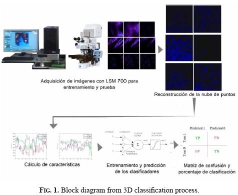
A. 3D image acquisition and reconstruction

The point clouds were obtained with the confocal laser scanning microscopy Zeiss LSM 700, which acquire 2D images from a fracture surface at different heights and stock them to generate a 3D block from the analyzed surface. As the height changes, a process of focusing and defocusing takes place in different regions of the surface. As a result, a discrimination of the material topology is achieved. Figure 2 displays the 3D reconstruction with the software Zen 2009.

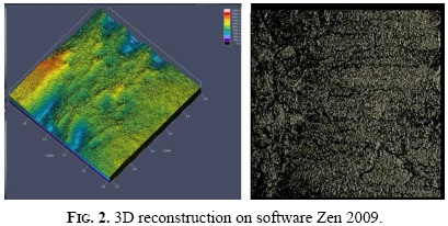
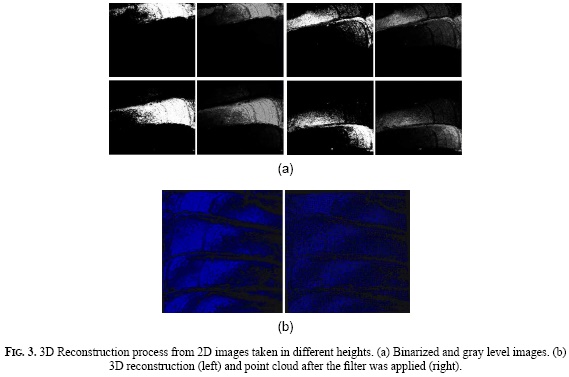
Due to software restrictions, it is not possible to save the 3D model of the surface; however, it is possible to obtain 2D images. From these images and using the C++ libraries, OpenCV, and Point Cloud Library (PCL), we built the point clouds of training and testing. To accomplish this, it was necessary to do an image binarization to determinate the points with information and save its gray level and its coordinates (x, y, z). Figure 3 shows a fracture surface with fatigue fracture, indicating the binarized and gray level images (Figure 3a). It can be observed that, as long as the height changes, new regions of the surface are focused. Figure 3b presents the reconstruction of a point cloud on the left, and the same cloud after we applied a voxel grid filter that reduces the quantity of points from 478.102 to 36.001 on the right.

B. Features and descriptors

Although a fracture mode differentiates from others by its marks and texture, these marks will not be found in all fractured mechanical elements, so we took the texture as the principal descriptor and used features that characterize it. Many 2D analyses have been expanded to 3D. It is important to highlight, as it is showed in [28] and [29], that, even though many methods have been proposed to describe texture, there is not yet a mathematical precise definition for this kind of problem due to the complexity and variation found in all fractured mechanical elements, so we real world textures are put through, such as scale, view point, light, among others.

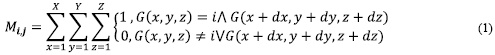
One of the most common methods to characterize textures is the Haralick's features [15]. This technique obtains a Gray Level Co-occurrence Matrix (GLCM) of an image and extracts features from its pixels. The GLCM is a spatial relation between two pixels located at a distance (d) and a direction(θ) between them. In order to take all the directions from a reference pixel into account, it is necessary to convert this matrix into a symmetric one by adding its transposed matrix. Finally, it is also necessary to obtain a probabilistic matrix with, where i is the number of rows or columns. There are many possible combinations for distance (d), but it is common to set d = 1 due to its computational simplicity [17]. In 3D analysis there are thirteen directions for each reference voxel, since this is surrounded by twenty-six neighbors. Mathematically, it is defined by (1), where G [X, Y, Z] is the gray level in the reference voxel, and G [X l dx,y dy,z l dz] is the gray level in the neighbor voxel [16].

Considering Haralick's features is one of the most used methods due to its computational simplicity in 2D texture analysis, it was transferred to a 3D space in some studies such as [30], where they proved that texture must be treated as a three-dimensional problem in order to keep the details of the structural elements.

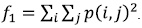
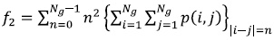
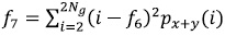
With the co-occurrence matrix, we calculated the features suggested in [15] and listed below, where p (i,j) is a probabilistic matrix, N_g the total number of gray levels on the image, and

- Angular second moment:

- Contrast:

- Correlation: 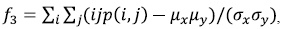where are the mean and the standard deviation of p_x and p_y.

- Sum of squares or variance:

- Inverse difference moment:

- Sum of average:

- Sum of variance:

- Sum of entropy:

- Entropy:

- Difference variance:

Difference entropy:

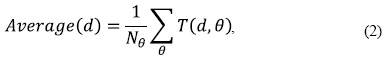
Finally, the average was calculated with (2) and the range with (3) in every direction, both are the input features to the classifier, where T (d, θ) is each feature and N_θ is the total number of directions.

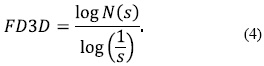
The fractal dimension allows to get useful information about the geometric structure in the image [18]. While the topological dimension is defined by an integer value that describes the dimension's number an object belongs to (1D, 2D, 3D), the fractal dimension uses real values to describe an object in terms of selfsimilarity and space occupancy [20]. The Differential Box Counting method is one of the most used to generate the fractal dimension. This method divides the object in voxels of size (s x s x s) and sets a gray level threshold; if the gray level of the reference voxel is over the value of the threshold, then this voxel counts plus one in the total occupancy. The fractal dimension is given by (4), where N (s) is the total number of voxels that contain the studied texture [19].

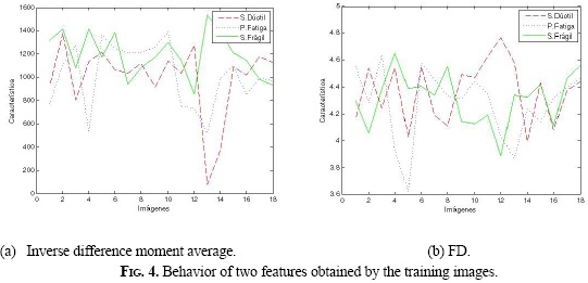
23 features were calculated in total (22 GLCM + 1 FD). Figure 4 exhibits the results for two of these features of the training images; figure 4a shows the average of the inverse difference moment, which is related to the homogeneity of the image (low values mean low homogeneity and vice versa), and figure 4b shows the fractal dimension of training images. The classification is difficult and requires the use of classifiers that allow to discriminate among classes. For this purpose, two classifiers where evaluated: ANN y SVM.

C. Confusion matrix

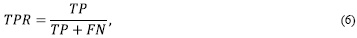
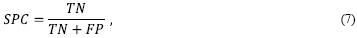
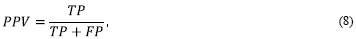
This matrix, which is developed for each class, allows to evaluate the classification algorithm. The cells in Table 1 are the true positives (TP), false positives (FP), false negatives (FN), and true negatives (TN). Among the marginal relations that can be obtained with this matrix are the accuracy (ACC), the sensitivity (TPR), the specificity (SPC) and the precision (PPV), given by (5), (6), (7) and (8).

D. Artificial Neural Networks (ANN)

The characteristics of the neural network implemented here are: training method: Backpropagation; stopcriteria: 1000 Iterations + Épsilon: 0.00001; Number of layers: three, one at the input (NC), one hidden (NO), and one at the output (Nclas); Number of neurons per layer: 23 in NC, 12 in NO, and 3 in Nclas; Activation

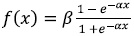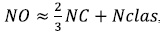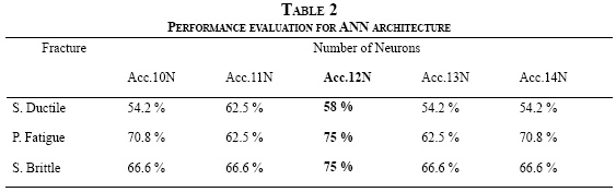
function: SIGMOID_SYM , , where β = 0.6 and α = 0.6. The total number of neurons on the hidden layer (NO) were selected taking into account that , where 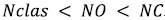Discriminability (i.e., how a classifier reacts faced with unknown datasets), using the confusion matrix and the accuracy, was used to evaluate the performance of the selected architecture (5). In Table 2, the performance analysis is showed according to the neural network in the hidden layer, with 12 neurons, in column Acc. 12N; the best performance is achieved taking into account two out of three failure modes.

E. Support Vector Machine (SVM)

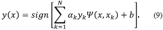
SVM is a discriminant classifier defined by a separating hyperplane, which means that given an input dataset, with its labels, the algorithm generates an optimal hyperplane able to categorize new samples [21]. Given a training set of N data points { y_k, X_k}^N k= 1, with X_k ∈ Rⁿ as the input pattern and Y_k ∈ R as the output pattern, as it is showed in (9), where α_k ∈ R positive and σ is a real constant[22],

a radial base was selected as a parametric function (RBF), as suggested in [21], 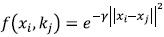with y= 5, and as a parameter for the optimization problem C 4 [23].

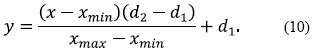
The input data for the classifier was previously normalized in order to avoid additional effects over the algorithm, using (10), where X is the value to be normalized, X_max Y X_min are the range of values in the vector, andd₁ y d₂ (([d₁, d₂] = [0,1])) are the range to do the normalization [24].

III. Results

The designed algorithm allows to classify fractures in mechanical materials by using computer vision techniques. In this section, the running test of this algorithm is presented using different performance metrics: the ROC space, the individual classification success index, and the Jaccard's coefficient. Additionally, a comparison between the results found here and the ones obtained by experts on the topic is presented.

A. Algorithm test

Previously, a classification of different pieces with the three kinds of fractures mentioned above was made using 2D images [27]. The results showed that the approach the authors used can be compared to the classification percentage made by an expert. In order to analyze the contribution of 3D point clouds, we decided to use the same training and testing pieces used in [27]; however, some of the pieces were too big or heavy to be analyzed with the microscope. Finally, 27 elements were selected for the training and 12 pieces for testing. For each piece, two regions of interest (ROI) were obtained. According to the obtained resolution and denoising, and the roughness of the piece, the microscope LSM 700 can take from 10 minutes up to a whole day to obtain a point cloud. For this research, an average of 25 minutes per ROI was selected considering the acquisition time and the resolution of the piece. Figure 5 shows three pieces, one for each fracture mode, with their 3D reconstruction, the classification given by the expert (one of the authors of this research), and the one given by the algorithm.

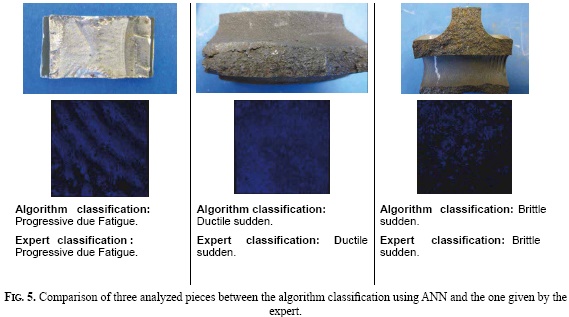
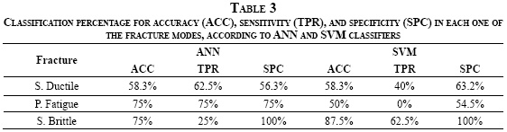
Table 3 presents the classification percentage for the 24 testing images, taking into account measures through the confusion matrix -equations (5), (6) and (7). It can be observed that, for surfaces with ductile sudden fractures and progressive fractures due to fatigue, the ANN classifier discriminated the true positives better than SVM, represented by the sensitivity relation TPR; in addition, for brittle sudden fractures, ANN classifier discrimination rate of true negatives was 100%, represented by the specificity SPC metric. In a global way, a good performance was achieved for brittle sudden and progressive fractures due to fatigue with 75% accuracy, and an acceptable performance for ductile sudden fractures, whose discrimination of true negatives is 56%. SVM discriminated among ductile and brittle fractures with a 58% and 50% accuracy respectively; however, the results for progressive fractures due to fatigue are not correct. The sensitivity TPR percentage is evidence of this.

B. Performance evaluation

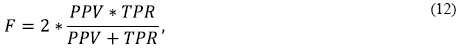
In order to evaluate the classifiers, we used: i) the ROC space (Receiving Operating Characteristic), where the sensitivity vs one minus the specificity is ploted (a perfect classifier must be located in coordinates (0,1) on ROC plane) [25]; and the metrics showed in [26]: ii) the individual classification of success index (ICSI) (11), and iii) Jaccard's coefficient (12). These methods depend on the marginal relations of sensitivity (TPR) (6) and precision (PPV) (8).

In Figure 6, the ROC space is displayed for the three kinds of fractures. With ANN, the randomness line is exceeded for the three modes and is much better than SVM with ductile and fatigue fractures due to fatigue do not exceed the randomness line-. However, SVM has a better discrimination for brittle fractures. For this kind of fracture, both classifiers had a discrimination of 100% for true positives.

Table 4 shows the results with the performance -even fractures indicators for the classification according to each failure mode. ANN performed better than SVM taking into account the three fracture classes, and SVM performed better for brittle sudden fractures.

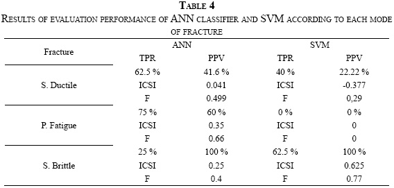
Even though the results obtained with 3D images in texture analysis for fracture classification are not better than the ones obtained by an expert or previous research using 2D images [27], it is interesting to analyze them. With SVM, it is possible to better discriminate brittle fractures; however, the accuracy percentages for the other two fracture modes are below 59%, and the ICSI has a negative or zero value; whereas, with ANN, an accuracy percentage of 58% for ductile fractures and 75% for the other two types was obtained. The three failure modes exceeded the randomness line in the ROC space, which proves that it is possible to classify these kinds of fractures by using 3D images. Furthermore, the initial hipothesis of using texture features in order to describe fracture surfaces is correct, which allows future works to aproximate themselves to generate an expert concept on the topic, testing different texture features and aqcuisition methods.

C. Expert validation

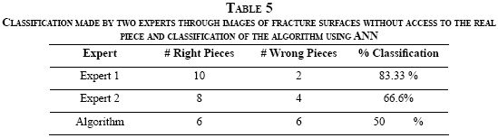
The research presented here had the support of three experts on materials engineering. The first expert, one of the authors of this paper, had physical access to the piece and made the initial classification of the surface fractures. The other two experts observed the 2D images of each piece and classified them into one of the three modes. The results obtained from the experts and the algorithm in terms of total pieces correctly classified are presented in Table 5. Considering that the total of testing pieces was 12, it can be observed that the classification range obtained by experts is between 83.3% and 66.6% These percentages allows to conclude that the fracture classification is not a simple problem and developing a computational tool that is able to do this classification would support the failure analysis.

IV. Conclusions

This research aims at classifying failure modes in: i) Ductile sudden fracture, ii) Brittle sudden fracture, and iii) progressive fracture due to fatigue, in order to support the fractographic study in failure analysis. To analyze the contribution of 3D images, the acquisition of the point cloud was made with the confocal laser scanning microscope Zeiss LSM 700 with a target of 5x, and representative ROIs were selected in order to be used as testing and training in the algorithm. In total, 27 pieces were used for training, 9 for each fracture mode, and 12 testing pieces, 4 for each failure mode. The first step to do a fractographic analysis corresponds to a visual inspection of the fractured surface, where the observation of particular features (marks and textures) is made to classify the flaw in one of the failure modes. In this work, the fractures were characterized based on their particular texture because there are no marks in every fracture surface, and descriptors were generated by the gray level cooccurrence matrix, Haralick's features, and the fractal dimension. The obtained results allow classifying the textures in ductile sudden fractures (58%) and brittle sudden and progressive fractures due to fatigue (75%), according to the accuracy percentage, and the performance evaluation with ROC space, which exceeded the randomness line of this space. The results were compared to the classification made by two experts on the topic. The experts observed the pieces through 2D images, with a classification of total pieces between 83% and 66%, which allows to conclude that the classification of fractured surfaces is not a trivial problem and that developing a computational tool could support failure analysis. The 3D study is significant and deserves to be evaluated. For future researches, we suggest to test different methods of characterization and use more point clouds for testing and training the algorithm.

References

[1] E. Espejo, "Fallas por fractura y fractografía," Notas de clase curso Análisis de Falla. Universidad Nacional de Colombia, Bogotá, 2013.         [ Links ]

[2] M. Ipohorski, Fractografía, Aplicaciones al Análisis de Fallas. Comisión Nacional de Energía Atómica, Buenos Aires, 1988.         [ Links ]

[3] H. Lauschmann and I. Nedbal, Auto-Shape Analysis of Image Textures in Fractography, Czech Technical University, Faculty of Nuclear Sciences and Physical Engineering, República Checa: Trojanova, 2002.         [ Links ]

[4] O. Mendoza, B. Vargas, and J. Mendoza, "Digital Processing of Fractographic Images for Welded Joints on Microalloy Steel API5L-X52 Aged," IEEE Latin America Transactions, vol. 11(1), pp. 172-176, Feb. 2013.         [ Links ]

[5] H. Lauschmann, O. Rácek, M. Túma, and I. Nedbal, "Textural Fractography", Image Anal Stereol, vol. 21(4), pp. S49-S59, Dec. 2002. DOI: http://dx.doi.org/10.5566/ias.v21.pS49-S59.         [ Links ]

[6] R. Ya. Kosarevych, O. Z. Student, L. M Svirs'ka, B. P Rusyn, and H. M. Nykyforchyn, "Computer analysis of characteristic elements of fractographic images," Materials Science, vol. 48(4), pp. 474-481, Jan. 2013. DOI: http://dx.doi.org/10.1007/s11003-013-9527-0.         [ Links ]

[7] O. Kolednik, S. Scherer, P. Schwarzbock, and P. Werth, "Quantitative fractography by means of a new digital image analysis system," in ECF13, Amsterdam, pp. 1-7, Nov. 2000.         [ Links ]

[8] M.P. Pradhan, R. Pradhan, and M.K Ghose, "Shape reconstruction of fracture surface for HSLA materials using photometric-stereo images," in International Symposium on Devices MEMS, Intelligent Systems and Communication (ISDMISC), 2011.         [ Links ]

[9] M. Khokhlov, A. Fischer, and D. Rittel, "Multi-Scale Stereo-Photogrammetry System for Fractographic Analysis Using Scanning Electron Microscopy," Experimental Mechanics, vol. 52(8), pp. 975-991, Oct. 2012. DOI: http://dx.doi.org/10.1007/s11340-011-9582-0.         [ Links ]

[10] J. Komenda, B. Maroli, and L. Höglund, "Recognition of patterns on fracture surfaces by automatic image analysis," Image Anual Stereol, vol. 21 (3), pp. 207-213. DOI: http://dx.doi.org/10.5566/ias.v21.p207-213.         [ Links ]

[11] K. Komai, K. Minoshima, and S. Ishii, "Recognition of Different Fracture Surface Morphologies using Computer Image Processing Technique," JSME international journal. Ser. A, Mechanics and material engineering, vol. 36(2), pp. 220-227, 1993.         [ Links ]

[12] K. Slamecka and J. Pokluda, "3D Analysis of Fatigue Fracture Morphology Generated by Combined Bending Torsion," in Advanced Fracture Mechanics for Life and Safety Assesments, Stockholm, 2003.         [ Links ]

[13] S. Stach, J. Cybo, J. Cwajna, and S. Roskosz, "Multifractal description of fracture morphology. Full 3D analysis of a fracture surface," Materials Science-Poland, vol. 23(2), pp. 577-584, 2005.         [ Links ]

[14] C. Leising, Fractography Analysis Using 3D Profilometry. Nanovea, 2010.         [ Links ]

[15] R. M. Haralick, K. Shanmugam, and I. Dinstein, "Textural features for image classification," IEEE Transactions on Systems, Man, and Cybernetics, vol. SMC-3(6), pp. 610-621, Nov. 1973.         [ Links ]

[16] Texture Directional -A Multi-Trace Attribute that Returns Textural Information Based on a StatisticalTexture Classification. Available: http://www.opendtect.org/500/doc/od_userdoc/content/app_a/text_dir.htm.         [ Links ]

[17] F. Tsai, C. Chang, J. Rau, T. Lin, and G. Liu, "3D Computation of Gray Level Co-occurrence in Hyperspectral Image Cubes," Lecture Notes in Computer Science, vol. 4679, pp. 429-440, 2007. DOI: http://dx.doi.org/10.1007/978-3540-74198-5_33.         [ Links ]

[18] L. Kenneth, Textured Image Segmentation. University of Southern California, 1980.         [ Links ]

[19] P. Bourke, Box Counting Fractal Dimension of Volumetric Data, 2014. Available: http://paulbourke.net/fractals/cubecount/.         [ Links ]

[20] A. R. Backes and O. M. Bruno, "Plant Leaf Identification Using Multi-scale Fractal Dimension," Lecture Notes in Computer Science, vol. 5716, pp. 143-150, 2009. DOI: http://dx.doi.org/10.1007/978-3-642-041464_17.         [ Links ]

[21] Introduction to Support Vector Machines. Available: http://docs.opencv.org/2.4/doc/tutorials/ml/introduction_to_svm/introduction_to_svm.html.         [ Links ]

[22] J. A. K. Suykens and J. Vandewalle, "Least Squares Support Vector Machine Classiffers," Neural Process. Letters, vol. 9(3), pp. 293-300, Jun. 1999. DOI: http://dx.doi.org/10.1023/A:1018628609742.         [ Links ]

[23] C. Staelin, Parameter Selection for Support Vector Machines. HP Laboratories Israel, 2002.         [ Links ]

[24] Redes Neuronales: de la teoría a la práctica, 2014. Available: https://www.mql5.com/es/articles/497.         [ Links ]

[25] T. Fawcett, "An Introduction to ROC Analysis," Pattern Recognition Letters, vol. 27(8), pp. 861-874, Jun. 2006. DOI: http://dx.doi.org/10.1016/j.patrec.2005.10.010.         [ Links ]

[26] V. Labatut and H. Cheril, Accuracy Measures for the Comparison of Classifiers" in The 5th International Conference on Information Technology, Jordanie, 2011.         [ Links ]

[27] M. X. Bastidas-Rodríguez, F. A. Prieto-Ortiz, and E. Espejo, "Fractographic classification in metallic materials by using computer vision," Engineering Failure Analysis, vol. 59, pp. 237-252, Jan. 2016. DOI: http://dx.doi.org/10.1016/j.engfailanal.2015.10.008.         [ Links ]

[28] A. Ahmadvand and M. Reza, "Rotation invariant texture classification using extended wavelet channel combining and LL channel filter bank," Knowledge-Based Systems, vol. 97, pp.75-88, Apr. 2016. DOI: http://dx.doi.org/10.1016/j.knosys.2016.01.015.         [ Links ]

[29] K. Hanbay, N. Alpaslan, M. Fatih, and D. Hanbay, "Principal curvatures based rotation invariant algorithms for efficient texture classification," Neurocomputing, vol. 199 (C), pp. 77-89, Jul. 2016. DOI: http://dx.doi.org/10.1016/j.neucom.2016.03.032.         [ Links ]

[30] E. Ben Othmen, M. Sayadi, and F. Fniaech, "3D Gray Level Co-occurrence Matrices for Volumetric Texture Classification," in 3rd International Conference on Systems and Control, Algeria, Oct., 2013. DOI: http://dx.doi.org/10.1109/ICoSC.2013.6750953.         [ Links ]