


 English (pdf)
 Article in xml format
 Article references
 Send this article by e-mail
 Cited by SciELO
  Cited by Google
  Similars in
SciELO
Similars in
SciELO  Similars in Google
 Permalink
I. INTRODUCTION
Although some of the horse morphological and locomotion characteristics can be perceived by the trained eye of an expert, the direct observation method lacks any quantitative and objective validity because it depends on the expertise, training, and judgment of each veterinarian. Moreover, several important aspects of the musculoskeletal system functionality, and the kinematic joint cannot be evaluated.
For horse motion analysis, different techniques, such as analytical photogrammetry 1, videometry 2, accelerometry 3, electromyography 4, and, rarely, mathematical modeling 5-7 have been used to help veterinarians and researchers to quantify movement. The first two techniques have several advantages, one of them is that the horse's body does not have to be instrumented and wired, and other is that they allow a qualitative and quantitative analysis of the horse gait. On the other hand, with accelerometers and electromyography is almost mandatory to instrument the animal, and the obtained results are mathematical values or electrical signals, which require a more complex processing for their interpretation. These techniques have proven to be useful for assessing the horse conformation [8], analyzing the gait in different breeds (Pure Spanish 9 Andalusian 10, Angloarabian, Warmblood 4, and others 11), determining the characteristics of movement at hand-led walk 2,9 and at different types of trot 12, analyzing the influence of speed and height on the withers 13, and studying the effect of different surfaces 14.
To our knowledge, there are few studies on mathematical modeling of equine movement, which allows different kinematic 5,15-16 and kinetic calculations 6,19. Some of the most relevant studies are based on 2D or 3D kinematics analysis of the interphalangeal 15 and metacarpophalangeal joints 16; in these studies, the authors only obtained ranges of motion for flexion/extension, adduction/ abduction, and internal/external rotation at walk and at trot. Furthermore, other authors have simulated the horse motion as a series of rigid articulated bodies 17,18, and have used coordinate systems for quantifying movements of the horse's digital joint 7, allowing a better evaluation of the kinematic and kinetic of all horse joints. In these studies, horse articular movement is very useful for characterizing its locomotion patterns, and for understanding its etiology, injury evolution and treatment, progress of training programs, etc.
The objectives of this study were to develop a mathematical model to generate and evaluate, qualitatively and quantitatively, the motion kinematics graphs of the most important horse joints, simulate the motion pattern for the fore and hind limbs, and, ultimately, assist scientists and veterinarians in an objective assessment of equine movement.
The main contribution of this paper is the construction of a mathematical model that is able to generate trajectory and kinematic curves of multiple horse joints, and to facilitate numerical comparisons of each horse curve, at each percentage of the gait cycle, with the normality band with ± standard deviation. Also, the user can display a 2D representation of the kinematics chain of the horse skeleton in his anterior portion, posterior portion, or entire skeleton, which will allow the user to better understand the phenomenon of the equine gait, and will eliminate the subjectivity of horse movement evaluations and diagnoses. This will let veterinarians to assess, diagnose, rehabilitate, and monitor the equine gait in a more objective, accurate, and scientific manner.
This paper is divided as follows: the first section explains the methodology to construct the mathematical model of joint kinematics of any horse, and its posterior validation; the second section presents the main results; and the final section closes with the main conclusions.
II. MATERIAL AND METHODS
A. Study subjects
Using computer-assisted videometry 9,19-20, we obtained the average values (x and y coordinates) of the movement of markers placed on skeletal references of 25 Andalusian horses at trot (Fig. 1).
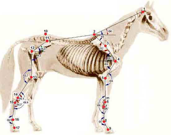
Fig. 1 Skeletal references (markers): 1. Wing of the atlas, 2. Withers, 3. Tuber of spina scapulae, 4. Greater tubercle of the humerus (caudal part), 5. Lateral collateral ligament of the elbow joint, 6. Lateral styloid process of the radius, 7. Proximal end of the metacarpal bone IV, 8. Lateral collateral ligament of the fore-fetlock joint, 9. Coronary band (forelimb), 10. Sacral tuber, 11. Coxal tuber, 12. Greater trochanter of the femur (caudal part), 13. Lateral collateral ligament of the stifle joint, 14. Lateral malleolus of the tibia, 15. Proximal end of the metatarsal bone IV, 16. Lateral collateral ligament of the hind fetlock joint, and 17. Coronary band (hind limb).
Figure 1 also shows the schematic representation of calculated joint angles. Angular variables are the following: 00 (neck inclination), 01 (neck angle), 02 (scapular alignment), 03 (shoulder), 04 (elbow), 05 (angle of radio vs. carpus), 05' (carpal angle vs. metacarpus), 06 (carpal angle), 07 (fore-fetlock), 011 (hip), 012 (stifle), 013 (angle of tibia vs. tarsus), 013' (tarsal angle vs. metatarsal), 014 (hock), 015 (hind fetlock), 017 (scapular inclination), and 018 (pelvic inclination).
B. Mathematical model approach
The mathematical model was set up representing the horse as a mechanical system of rigid bodies articulated by simple joints (Fig.1). The model was developed using an inverse kinematics analysis, which employs basic principles of the kinematics of rigid bodies (Fig. 2).
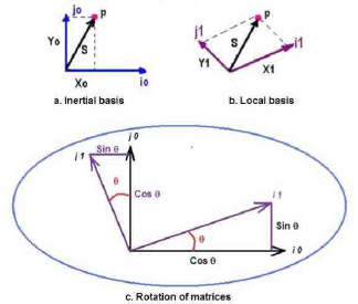
Fig. 2 Representation in the plane of a) inertia base, b) local base, and c) the rotation of matrices.
In the mathematical model, there is an external inertia base fixed on the origin (0,0), and there are 15 local mobile bases located in anatomical points (Fig. 3). These bases are rotated and move a distance (longitudinal to each segment) by means of inverse kinematics equations to calculate the angular movements.
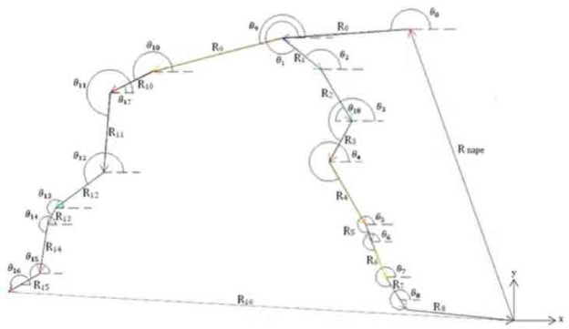
Figure 3 also shows the two main kinematics chains that represent the forelimb (Rnape+R0+R1+R2+R3+R4+R5+R6+R7) and the hind limb (Rnape+R0+R9+R10+R11+R12+R13+R1 4+R15), and that were used to calculate the inverse kinematics. The vectors, Rnape, R8, and R16 were used to complete the kinematics chains associated with fore and hind limbs, respectively.
Based on the representations shown in figure 2, the following correlations of the coordinates can be obtained:
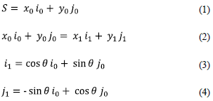
Thus, the general position equation is obtained.
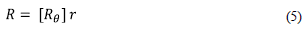
Where:
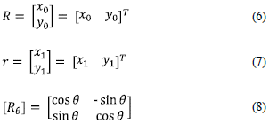
R[θ] is the rotation matrix.
The position of the mechanism was analyzed from a passive point of view, with a coordinate system having an inertia base fixed to the ground (external), and mobile local bases located on the skeletal references, united to the joints of the mechanism (aligned in X) (Fig.3), for which, a related base change matrix was built (8) 21. The vectors employed for this biomechanical system are presented in Table 1.
Table 1 Mathematical proposal for the vectors of the fore and hind limbs employed in the mathematical model (ri are the lengths of the segments)
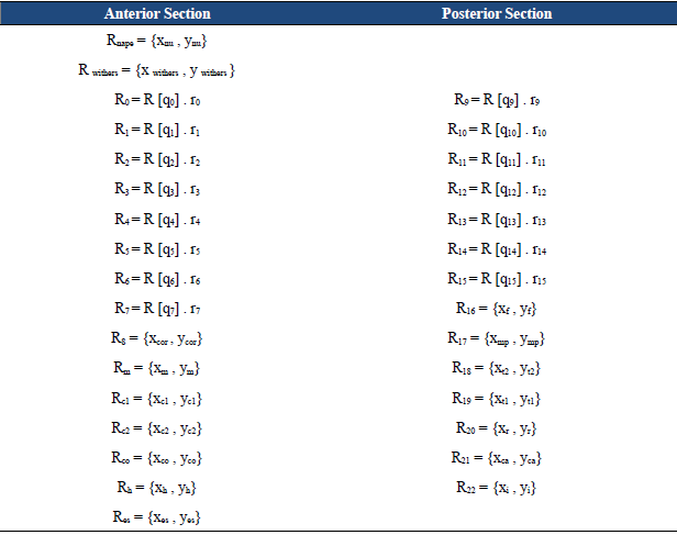
All vectors in Table i are related to each other to build the kinematics chains (Fig. 3), which, along with the rotation matrices, the vector magnitude, and the coordinates of each point, allow to calculate the angular movements by means of inverse kinematics.
C. Mathematical processing of information
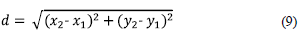
Calculation of body segments length. The length of the body segments (L0 - L15) was calculated using the coordinates (x, y) of each marker in the first frame of the stride of the experimental data, and using the equation (9) of distance between points.
Calculation of initial angles. Markers on the skeletal references (Fig. 1) were used to define the angular variables of the system (at the initial time). These angles were calculated using the scalar product (10) and the coordinates (x, y) of the involved points 3 and 4 (Fig. 1), according to the protocol.

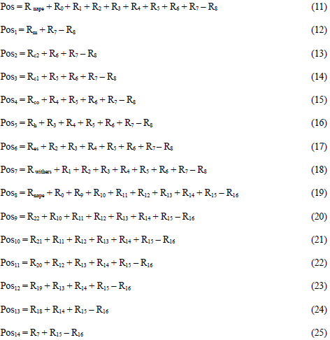
Programming the mathematical model to calculate joint kinematics. To calculate graphs and simulate the angular movements of each joint, we developed a script using the Mathematica® software, and incorporated the following items: the rotation matrices (8), the trajectory values (x, y coordinates) of each point throughout the gait cycle, the lengths of each body segment, and the angles of each segment vs. the horizontal axis in frame 0 (initial frame of the gait cycle video), the mathematical approach of the vectors (Table 1), and the loop equations of each kinematics chain (11 - 25).
• Least Squares Method.
Because the system is nonlinear, with more unknowns than equations, a numerical analysis was performed using the mathematical optimization method created by Powell 22 and Fletcher23) here, given a set of coordinates (xk, yk), where k = 1,2, ..., n., and fj, with j = 1,2, ..., m, a basis of m functions, linearly independent, we found a function f linear combination of basic functions, such as f (xk) » yk, that is:

This method is measured and minimizes the error in the whole approach, making it necessary to find the m coefficients cj that make the approximant function f(x) the best approximation to the points (xk, yk). The approximation process using the least square method (the steepest descent method) is based on the minimization of the mean square error (or equivalent), so we should minimize the filing of this error. The quadratic error is defined in (27).
For each loop equation (11-25), the function that best approximated the experimental data was calculated, according to the criterion of minimum square error (implemented in Mathematica®). With the sum of the objective functions of each loop equation (28), a total objective function (29) was generated, which then was used to calculate the angular movement of the segments during the gait cycle.

Where i = 0, 1, 2, ... , 14.

Posteriorly, to calculate and graph the variation in movement of the whole system of joint angles, we established correlations between angles; for example, the elbow joint angle was determined through equation (30) that correlated with the angles (not joints) q4 and q3.

D. Validation of the mathematical model results
We compared the results obtained by the mathematical model with those obtained by a Digital Video
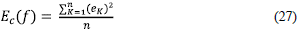
Morphometric System (DVMS) 9, for the same horses by the 2D videography analysis system. For every angular variable, the numerical difference between the experimental and the theoretical averages was determined for every 10 % of the motion cycle, and the average and standard deviation of these differences were calculated (Table 2). In addition, we visually inspected and compared the patterns graphs of the joint angle values vs. time (% stride), obtained by the mathematical model and those obtained by Digital Video Morphometric System (Fig 4).
Table 2 Average and standard deviation of the differences between the experimental average (videometry) and the theoretical average (mathematical model) for fore and hind limb angular variables
| Average (°) | Standard Deviation (°) | |
|---|---|---|
| Neck Inclination | 0.43 | 0.3 |
| Scapular Inclination | i.57 | 0.6s |
| Shoulder Kinematics | 2.13 | i.2i |
| Elbow Kinematics | 3.9s | 2^ |
| Carpal Kinematics | 1.s3 | 2.5s |
| Fore Fetlock Kinematics | 3^7 | 2.56 |
| Fore Retraction - Protraction Angle | 0.017 | 0.012 |
| Height of the Fore Coronary Mark | 0.0029 | 0.0024 |
| Hip kinematics | 4.3 | 2.44 |
| Pelvic Inclination | 1.s | 0.61 |
| Stifle Kinematics | 5.7s | 5.3 |
| Hock Kinematics | 0.05 | 0.07 |
| Hind Fetlock Kinematics | 9.12 | 9.12 |
| Hind Retraction - Protraction angle | 0.02 | 0.01 |
| Height of the Hind Coronary Mark | 0.006 | 0.002 |
III. RESULTS
We designed a 2D-real-scale representation of an articulated rigid body system, with some of the most significant "body segments and joints", by means of the mathematical model. In addition, we obtained graphs of the joint angle values vs. time for the trajectories of the main markers (coordinates x, y).
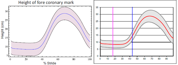
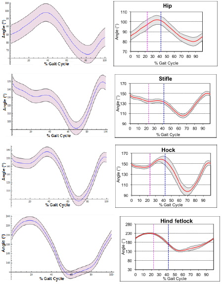
For the 25 horses at trot, we generated graphs of the joint angle value vs. time for the angular variables of the fore and hind limbs (Fig. 5). Additionally, we calculated the standard deviation and maximum and minimum values of the angular variables for each angle. With these data, the software generated three normality bands (Fig. 6), which allowed us to make a quantitative and objective assessment of the equine locomotion pattern.
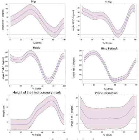
Fig. 5 example of joint angles vs. time (% stride) graphs of hind limb (average ± standard deviation) for 25 horses at trot obtained by the mathematical model. Shadow areas are one standard deviation from the mean curves.
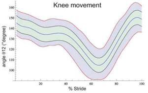
Fig. 6 joint angles vs. time (% stride) graphs for the stifle (012) obtained by the mathematical model. Normality bands with mean values (blue line), ± standard deviation (black line), and ± minimum and maximum values (pink lines). The green zone represents the normality band.
For a better understanding of the equine movement, the fore and hind limb motion was simulated both separately and assembled (together), and displayed to the user (Fig. 7). During the simulation, the model allows to represent the trajectories of a specific, several, or all markers. It is also possible to check the normality or abnormality of the movement pattern through the full motion cycle.
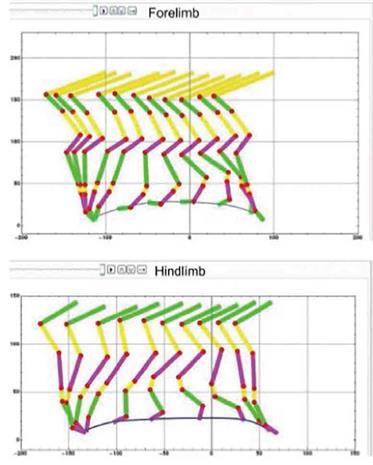
Fig. 7 Schematic representation of the simulation for fore (a) and hind (b) motion of a trotting horse (Sequences and trajectories of margo coronalis).
For every angular variable at every 10 % of the full motion cycle, the numerical difference between the experimental and the theoretical averages of each joint movement was calculated, and the results of this model were validated numerically and graphically.
The mathematical methodology used (kinematics chains), not only generated kinematics curves of the main joint variables (Fig. 4 and 5), but also created curves of other angular variables. The graphics obtained in this study could be helpful for future studies for analyzing normal and abnormal (lameness) equine movement.
In this study, we used the angles of the body segments with respect to the horizontal axis for the position equation (Fig. 3). For a better understanding of the graphical representation of the results, in which the traditional extension-flexion concept is maintained, it was necessary to make the conversions.
The numeric differences between the experimental (videometry) and the theoretical (mathematical model) averages were small, except for the hip (4.3°), the stifle (5.78°), and the hind fetlock (9.12°) joints. However, if these values are compared with the values for the full range of movement, the differences do not seem to be great (Table 2 and Fig. 4). Under visual inspection, the experimental and theoretical graphs were very similar in their starting values, and in their pattern shape (Fig. 8).
IV. CONCLUSIONS
Thanks to the mathematical model generated to analyze the kinematics in 2D of the horses at trot, we were able to correctly generate kinematics curves of the most important joints, and other angles of interest for veterinarians that are impossible to observe to the naked eye. In addition, we were able to recreate the gait or trot of the horses as a skeleton formed by articulated rigid bars. The trajectory graphs and the numerical results for angular variables (average angles, maximum, minimum, and angular motion range) were determined and simulated in 2D. The model generated allowed a qualitative and objective analysis of the equine movement (removing the subjectivity in assessing movement patterns), the control of rehabilitation and training programs, and the effective verification of the pharmacological or surgical treatments, among other factors.
The mathematical model of equine biokinematics can be used in two directions: one, by extracting the trajectories and the horse angular movement to understand and evaluate the kinematics of the joints, and two, by employing trajectories and joint angles in the field of robotics, in order to induce movements in quadruped robots to simulate the movement of electromechanical devices and quadruped animals. Graphic animations by computer are also useful for studying the morphology and movement of equines and other animals in the video game and movies industries, and in many other fields.
The numeric differences between the experimental and theoretical averages, and the average and standard deviation for the differences in every angular variable were small, except for the elbow and hip that presented a slightly greater variation. The reason for this may be that while in the mathematical model the lengths of the body segments are constant, in the experimental method these lengths are variable because they were calculated at every time sequence. The shape pattern of the graphs for the angular variables obtained by the model agrees with those previously reported in the literature for trotting horses.
Knowing how the major joints move in a horse is very useful for understanding the etiology, course, and treatment of injuries in tissues. Having a good mathematical model of horse motion will help future research on horse kinematics at different gaits, inclinations, speeds, breeds, surfaces, with real, simulated, or induced lameness, etc.

