


 English (pdf)
 Article in xml format
 Article references
 Send this article by e-mail
 Cited by SciELO
  Cited by Google
  Similars in
SciELO
Similars in
SciELO  Similars in Google
 Permalink
I. Introduction
The capacitated vehicle routing problem (CVRP) is a well-known problem in transportation proposed in 1959 [1]. It is defined over an undirected graph G(V,E), where V=v 0,...,vN is a set of vertices and E=(vi,vj ):vi,vj ∈V,i < j is a set of edges. There is a symmetric matrix C=[cij ] that correspond to the travel costs along edge (vivj ). Vertex v 0 represents the depot where there is a homogeneous fleet of m vehicles with capacity Q. A set of customers V\v 0 with a non-negative known demand di must be served. A solution to the CVRP consists of m delivery routes with some specific conditions. Each route must start and end at the depot. Each customer must be visited once by exactly one vehicle. The summation of the demands of the customers in the same route, must be less than or equal to Q. A different approach where the demand corresponds to items that must be collected from the customers leads to an equivalent problem. The classic objective is minimization of total travel costs [2].
The previous definition holds for the deterministic CVRP, however it is expected that in the real world one or more of the elements of the CVRP will be uncertain. Such elements are included in the models in the form of stochastic parameters. This variant of the problem became known as stochastic (capacitated) vehicle routing problem (SVRP or SCVRP) [3, 4].
Delivery reliability defined as the on-time delivery of products and services is a major competitive arena for many companies [5]. The travel time between two customers may be affected by the congestion in the road and other eventualities, such as accidents, making the CVRP with stochastic travel times a relevant problem to study. This paper deals with a stochastic multiobjective vehicle routing problem with soft time windows (TW). The penalty for servicing the customers outside the time windows is included as objective, in addition to the traditional minimization of the total length. The travel times are assumed to be stochastic. This problem is known as the VRP with soft time windows and stochastic travel times (SVRPSTW).
Real-world transportation planning is a multiobjective problem [6]. It can be expected that including additional relevant objectives into the model will make it more realistic. In a multiobjective optimization problem (MOP) several functions are optimized (minimized or maximized) subject to the same set of constraints. As a general rule, no single solution can minimize all objectives simultaneously. Instead of that, a solution to a MOP is given by a set of solutions, which are called tradeoff solutions [7], Pareto optimal solutions or Pareto Set [8].
The tradeoff solutions consist of the set of non-dominated solutions. A solution y with objective function values (f 1(y),f 2(y),...,fn (y)), dominates a solution z,y<z, if and only if, the solution z does not perform better than y in any objective function, but it performs worse in at least one.
When dealing with stochastic MOP the dominance may be evaluated in different ways [9], the expected values of the objective functions are used here to compare. A multiobjective model for the SVRPSTW was formulated in [5]. However, their solution approach was not entirely multiobjective. In contrast, we attempt to approximate the Pareto set.
A. Problem definition
A multiobjective approach to the CVRP with soft time windows and stochastic travel times (SVRPSTW) is found in [5]. In SVRPSTW the demand is known in advance, and there is a deterministic service time and a time window [eili ] associated with each customer i. Starting service outside the time window is allowed at a cost, either for earliness or lateness. The problem is modeled as stochastic programming with recourse (SPR), the recourse being the cost for servicing outside the time windows. The development of the mathematical model to the problem is explained in detail in [5].
Even though the problem is modeled as a multiobjective problem, just two potentially Pareto solutions are found. The three objective functions are combined into a weighted single objective which is later minimized by the tabu search algorithm. Tests were performed using two different sets of weights, one solution is found in every case.
A bi-objective reformulation of the SVRPSTW is presented here, where both the expected total distance and the expected penalty cost (for starting the service outside the time windows) are minimized. The Number of vehicles is given as parameter, in principle it is possible to use the value found in [5]. However, it is possible to set different values to the number of vehicles and solve the bi-objective problem for each value. In that case, the obtained sets of solutions will approximate the Pareto set to the original SVRPSTW.
The obtained solution sets are compared against the solutions presented in [5]. The fact that the solution to the problem is presented in a form of approximation to the Pareto set, becomes one main contribution of this work. Since no previous attempts have been made to approximate its Pareto set. Another contribution is the algorithm that succeeds in finding such approximation.
B. Travel time and closed-form expressions for the penalties
The travel times are considered to follow a shifted gamma (α,β,δ) distribution, where α is restricted to take only integer values. This condition on the travel time allows the exact penalty computation, at the cost of generality. The arrival time at customer i, τi, is equal to the cumulative travel times plus the sum of the service times of all preceding customers. The earliness penalty at customer i, Ξi, was expressed in [5] as in Equation (1).
 (1)
(1)
Where  ,
, 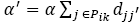 , α∈ ℤ+,β∈ℝ+,δ∈ ℝ+
0, α is a weight coefficient, j' is the customer immediately following j in route k, Pik
is the set of customers served before i in route k.
, α∈ ℤ+,β∈ℝ+,δ∈ ℝ+
0, α is a weight coefficient, j' is the customer immediately following j in route k, Pik
is the set of customers served before i in route k.
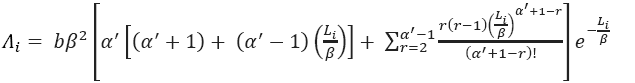
On the other hand the tardiness penalty at customer i, Λi , can be expressed as in Equation (2).
 (2)
(2)
Where  , b is a weight coefficient.
The weight coefficients a in earliness and b in the tardiness penalty are assumed to be equal to one. The penalty for serving the customers outside the time windows is assumed to be a quadratic loss function, in that way, larger deviations will cause progressively larger losses. If the service at customer i starts at time τi and τi <ei , the earliness penalty will be equal to (ei−τi )2. The lateness penalty would be equal to (τi−li )2, in case that τi >li . A discussion on other alternatives for penalty functions and their mathematical expressions can be found in [5].
The waiting time before each customer, including the depot, is a decision variable. So once a vehicle arrives to a customer, it can immediately serve the customer or it can wait. In [5] this decision is done in a post processing procedure, since the main algorithm assumes zero waiting time.
C. Literature review
There are several variants of the SVRP. One of such variants is modeled using the times as stochastic parameters. It can either be the travel times, service times or both. In [10] a CVRP with soft time windows and stochastic travel and service times was solved by means of a tabu search algorithm. A variant of the previous problem, without stochastic travel times and no time windows, was presented in [11], a generalized variable neighborhood search (GVNS) was proposed to solve it. In [12] the CVRP with stochastic travel time and simultaneous pick-ups and deliveries was solved using a scatter search heuristic. Other methods have been used to solve a variant of the last problem see [13, 14]. In [15] a VRP with stochastic travel and service time is described. A robust CVRP with deadlines and travel time/demand uncertainty is studied in [16]. For a more detailed summary on different SVRP, see [3, 17, 18].
There is scant literature on multiobjective SVRP, to the best of the author`s knowledge examples can be found in [5, 19, 20, 21]. A multiobjective approach of the CVRP with stochastic demands (CVRPSD) was formulated in [21]. In [20] the CVRPSD is not explicitly presented as a bi-objective problem, but a tradeoff between the total expected cost and the probability of the solution suffering a route failure (reliability) is taken into consideration. An extension of the CVRP including location, allocation and routing under the risk of disruption is introduced in [19]. A multiobjective CVRP with soft time windows and stochastic travel times (SCVRPSTW) is found in [5].
II. Methods
Evolutionary algorithms (EA) have been used for dealing with different types of VRP. In [22] an EA was used for solving a multiobjective CVRP. Memetic algorithms have been used to deal with different versions of the stochastic VRP [23, 24]. In [21] an EA was used to approximate the Pareto set of a multiobjective SVRP. This may be an indication of the potential of the EA for dealing with multiobjective VRPs and SVRPs.
The target aiming Pareto search (TAPaS) algorithm [8] takes an approximation PSappr to a Pareto set and improves it by using a tabu search. An algorithm that follows the same principle as TAPaS, is proposed here, where starting from the approximation obtained from a EA, a local search procedure is applied to improve the quality of the solution. An implementation of the NSGA-II [25], using particular characteristics for the CVRP [26] will be used as EA.
A local search that uses different neighborhood structures, as in generalized variable neighborhood search [11] is applied after the EA. Different neighborhoods are used to attempt to optimize the different objectives and will be applied sequentially. Moves leading to solutions that dominate the incumbent solution are accepted. In [11] the best improvement rule is applied, in this case the application of such rule can be complex and expensive, so the first improvement rule is applied here.
A. Construction of initial solutions
A set of initial solutions is required. We propose a simple deterministic construction heuristic. Most likely high quality solutions will not be obtained, but it can be one step ahead of the randomly constructed set. This heuristic is based on the one used in [27], which is a modified version of a classical insertion heuristic proposed in [28]. An initial diverse set of VRP solutions is constructed with priority shifting from TW penalty to total length. This is achieved by solving a sequence of deterministic hard time-windows problems, where the original (soft) time windows are extended by a varying slack parameter while the distance is minimized as a single objective.
B. Evolutionary Algorithm (EA)
The evolutionary algorithm used here is an implementation of NSGA-II [25], where two crossover operators are used, Split [26] and RBX [29]. The mutation operator will be Or-opt as in [8, 22]. The move that dominates all the others is accepted. The comparison is done among the neighbors, without considering the initial solution. If no move dominates all the others, among the non-dominated moves, the selection will be done comparing the normalized values of the objective functions.
A 2-opt procedure is included as local search. Such procedure has been used before in [8, 22], but here it deals with two objective functions and include the domination criteria. Given two possible moves, the first lead to solution y and the second to solution x, if they are non dominated, ⱻ A ⊂{1,2,...,n}: ∀i ∈A fi (y)<fi (x), and ⱻ B ⊂{1,2,...,n}: ∀j ∈B fj (y)>fj (x), will be preferred if Σ i∈A (1−fi (y)/fi (x)) > Σj∈B (fj (y)/fj (x)−1). If there is no inequality, one solution is selected randomly.
C. Local search
Once the EA has been executed, every found potentially non-dominated solution is subject to a local search procedure, based on the GVNS heuristic in [11]. In the local search just moves that lead to a solution that dominates the incumbent solution are accepted.
The local search (VNS) performs the search using different neighborhood structures. As in [11], there are inter- and intra-route operations. However, the number of neighborhood structures used in the local search is lower, since the computational requirements are higher. For accepting the moves, the first improvement rule is applied. It assumed that a move will improve the incumbent solution if it leads to a neighbor solution that dominates it or to a solution that does not dominate it, but the improvement in one of the objectives is greater than the deterioration in the other one, as percentage of the current values. A random inter-route swap move is used as a shaking operator. The different neighborhoods are: intra-route insertion moves, intra-route swap moves, inter-route swap moves and Or-opt procedure.
D. Post-optimization
The waiting time at every node, including the depot, is a decision variable. Departure from the depot can be postponed as well as the beginning of the service at every customer. In [5] this decision is done in a postprocessing procedure, since the main algorithm assumes zero waiting time at customers, not at the depot. Waiting times at the depot are computed based on the expected travel times to the first customer in the routes. If the expected travel time from the depot to the next customer is shorter than the early TW parameter associated to such customer, the waiting time at the depot will be equal to the difference, zero otherwise. The postprocessing procedure may change that value. The generalized reduced gradient method is used to deal with such variables in [5]. In our approach the decisions regarding waiting times are also part of a postprocessing procedure. We rely on the quasi-Newton Broyden-Fletcher-Goldfarb-Shanno (BFGS) algorithm [30] in Scilab for doing such procedure, since we find very convenient to access it from C++ and it is an open source package.
E. Solution evaluation
The equations used by [5] to compute the exact value of the penalties and previously described in Section 1.2, require massive computation, since they deal with transcendental functions and operations with large integers. Such operations can eventually lead to an integer overflow. As a mechanism to avoid such condition, natural logarithm transformations are used, which increases the computational requirements. An evaluation strategy is proposed looking to overcome such difficulty. The evaluation of the solutions is done in different ways along the search process, an idea borrowed from [31]. Let us say that the EA has a maximum number of generations GEN. This total number of generations is divided into three parts from zero to gen 1, from gen 1 to gen 2 and from gen 2 to GEN. During the execution of the algorithm, while running within the first part of the generations, the solutions and the moves are evaluated using deterministic values, and the travel time from a customer i to a customer j is given by the expected value (αβ+δ)dij . In the second part of the generations the solutions and moves are evaluated using sample scenarios. And only in the third part of the generations, the exact value for the expected penalties is computed using the closed-form in equations 1 and 2. Lookup tables were implemented for some of the computations, as a mechanism to reduce the processing time.
Using scenarios for evaluating the solutions has an additional advantage in a different context. If the expected values of the objective functions are unknown, this can be approximated with scenario evaluation. The values would not be exact, but the algorithm becomes independent of the probability distributions of the stochastic parameters. This is out of the scope of this work, however, it is an aspect worth of comment.
F. Test environment
The same instances as in [5] are used. These are a modified version of Solomon instances [28]. Four base test problems are used, R101, R102, R103 and R109. Four different sets of parameters for the travel time probability distribution (α, β and δ) are used with each instance, (1.00, 0.25, 0.75), (1.00, 0.50, 0.50), (1.00, 0.75, 0.25) and (1.00, 1.00, 1.00), identified as S1, S2, S3 and S4 respectively. The number of vehicles is also predefined and is set to be the same as in [5], which means that there may be two versions of the same instance, with a different number of vehicles available. As an illustration, we can say that the instance R101-S3-18V, corresponds to the instance R101, where the parameters of the travel time probability distribution are given by the set (1.00, 0.75, 0.25) and there are 18 vehicles available. In total there are 27 instances for computational experiments. Ten different runs per instance were performed.
The parameters of the algorithm were tuned by means of preliminary testing. A subset of eight test instances was used for the tuning. Each instance had 100 customers, but different set of parameter for the travel time probability distribution and different number of vehicles. Different values were tested for the parameters and these leading to better results, in the first 100 generations, were selected. In some cases, as in the number of generations or population size, also the execution time was taken into account. Regarding the number of generations, several values were tested, including 100. Unless stated otherwise, the values given to these parameters are: number of generations for the NSGA, GEN=300; population size for NSGA, 150; probability of applying RBX crossover operator, probco =0.5; probability of mutation, probmt =0.4; number of iterations for VNS, 100; randomization factor of construction procedure, lf =5; number of generations evaluated deterministically, GEN 1=0.5GEN; number of generations evaluated by scenarios, GEN 2−GEN 1=0.25GEN; number of scenarios, 20 (stability tests were carried out [32]); and maximum number of consecutive customers to move in the Or-opt procedure, 3. All computational experiments were conducted on a computer with processor Intel (R) Xeon (R) CPU E31270 @ 3.40 GHz and 16.0 GB of RAM.
III. Results and discussion
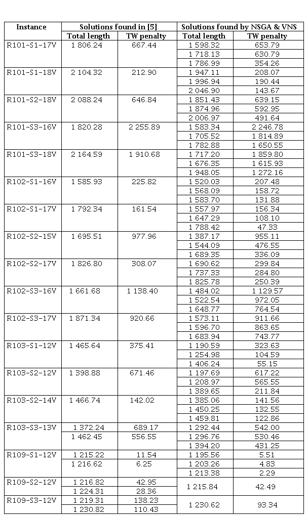
The suggested approach (NSGA&VNS) can find solutions that dominate the solutions reported in [5]. In 12 out of 27 instances such solutions are found even without applying the postprocessing procedure. Once the postprocessing procedure is applied, solutions dominating the ones in [5] are found in 18 out of 27 instances, however in one of the instances, R109-S3-12V, just one of the two solutions is dominated. Results are presented in Table 1. It is emphasized that the NSGA&VNS solutions in Table 1 do not correspond to the approximation of the Pareto set, these solutions are only a subset of the solutions that NSGA&VNS is able to find.
The instance R103-S1-14V is an example of the instances where solutions dominating the solution reported in [5] were not found. Figure 1 shows a section of the Pareto set approximation including both, NSGA&VNS approximation and the solution in [5]. On the other hand, the Figure 2 shows a section of the Pareto set approximation for the instance R101-S2-18V, where it is possible to see that the solution in [5] is dominated by solutions in NSGA&VNS approximation.
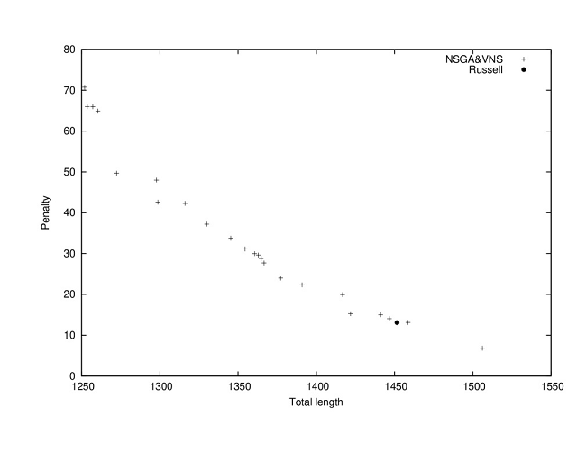
Fig. 1 Our approach finds solutions that do not dominate solution found by [5] in instance R103-S1-14V.
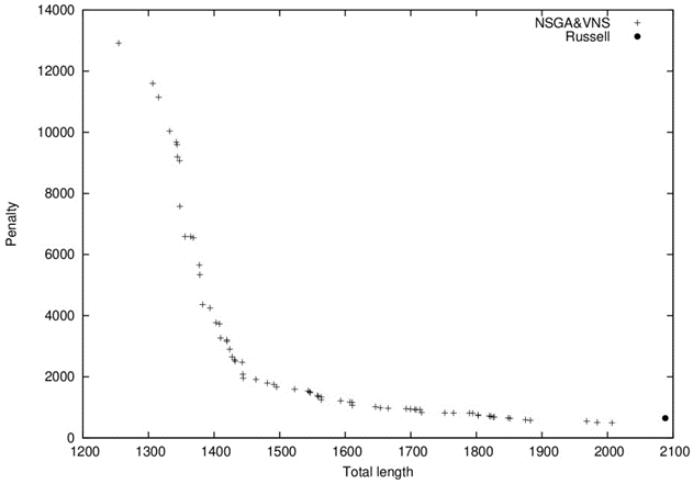
Table 2 Running time (in minutes).
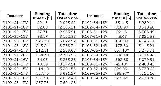
*The algorithm finds two independent solutions. Time computed by adding both running times.
The running time of NSGA&VNS is much longer than in [5], as it can be seen in Table 2. This can be explained by the fact that while in [5] one solution, at most two, are found per instance, we find an approximation to the Pareto set. As expected, the quality of the Pareto set approximation is improved by the postprocessing procedure. Using the average value of the S metric [22, 33, 34] to compare the two approximations to the Pareto set, before and after the postprocessing procedure, it was found that the average improvement over all instances is 0.96%. Russell and Urban [5] reported average improvement above 20%, but such improvement is measured over the objective function value; in contrast, the improvement of the Pareto set is measured here.
A. Impact of NSGA and VNS procedure on the results
A second set of experiments was conducted looking to assess the impact of the NSGA and the VNS procedure in the quality of the obtained solutions. All instances were used in these experiments and ten runs per instance were performed. Three different configurations of the algorithm were compared: the original algorithm described in the former Section (NSGA&VNS) and two algorithms, each consisting in one of the main components of the previous, NSGA and VNS procedure. The running time of the NSGA&VNS was reduced by setting the number of generations for the NSGA component to 30 and the iterations for the VNS to 10. The number of generations of the algorithm consisting of just the NSGA was set to 140, so its running time becomes not shorter than the one used by NSGA&VNS. For the case of the tests using the VNS procedure, the number of iterations was set to 120.
Results were compared using the S and the C metric, as in [22]. It is worth remarking that given two sets of solutions (R, X), the C metric measures the ratio of solutions in X weakly dominated by solutions in R. Using the average value of the metrics, NSGA&VNS performs better than NSGA in 15 out of 27 cases. In six instances is not possible to say which configuration has a better performance since the two metrics are contradictory. On the other hand NSGA&VNS performs better than VNS in 17 out of 27 instances. In eight cases the two metrics lead to contradictory conclusions.
It was observed that VNS is able to find extremal solutions, that do not necessary dominate the solutions found by the other two configurations, but in some cases are good enough to dominate the solutions found in [5]. The NSGA provides a denser set of solutions, which is reflected positively in the S metric. In the NSGA&VNS the solutions found by NSGA are used by VNS afterwards. The latter can improve the solution set by either finding dominating solutions or improving the extremal solutions, outperforming the solutions sets found by NSGA and VNS when executed individually. In conclusion, these experiments indicate that the combination NSGA&VNS works better than each individual method.
IV. Conclusions
The Pareto solutions to a known multiobjective SVRP were approximated for a first time. Obtained results were compared to previously reported individual potentially Pareto solutions. In most of the tested instances, the suggested approach is able to find solutions that dominate the existing solutions, in addition to a wide range of solutions where priority shifts from one objective to the other.
The suggested approach provides good results in most of the tested instances, but still there is room for improvement and several directions can be applied for further research. The efficacy of our approach is decreased when dealing with problems that present a high coefficient of variation. A different construction of initial solutions or local search operators could be adapted to deal with this particular type of instances. A different aspect to consider is the running time, the closed-form expressions for computing the expected value of the TW penalties require a large number of algebraic operations. Perhaps such expressions could be approximated using a method more efficient than the scenarios, but less demanding than the closed-form. Taking waiting times into consideration during the execution of the main algorithm is likely to improve the solutions. This, however, will increase the complexity of the problem. Further work can be done dealing with such complexity and testing the impact on results.

