


 Inglês (pdf)
 Artigo em XML
 Referências do artigo
 Enviar este artigo por email
 Citado por SciELO
  Citado por Google
  Similares em
SciELO
Similares em
SciELO  Similares em Google
 Permalink
I. INTRODUCTION
The abstraction of reality has long become an essential means of thinking and expressing, being indispensable in reasoning, knowledge, and interrelation. Abstraction has been spread in terms of machines (Machine Learning), where reality is abstracted through a careful analysis of all variables, to the point that the machine is able to predict based on the incoming data. Support Vector Machines (SVM) is one of the most widely used algorithms to perform prediction tasks in different scenarios. One of the main features that make it a good predictor is the possibility of finding nonlinear patterns in the data through the Kernel trick, which takes the original feature space where the data are not linearly separable to an infinite dimensional Hilbert space where the data are linearly separable [1]. In that sense, traditional Kernel functions such as linear, polynomial, and Gaussian (rbf) Kernel have been used. However, it is possible to improve the results of the algorithms using alternative kernel functions [2].
In 2040, total energy demand in the world will increase by 30% and most of this consumption will come from developing countries. In addition, 37% of electricity generation is expected to come from renewable sources, especially wind and solar. So then, solar energy is retaken, allowing electricity to be obtained completely free and renewable, in this sense, photovoltaic solar energy is the electrical energy generated by the photovoltaic effect that occurs when solar radiation falls on a photovoltaic panel[3]. Hence, there is a clear worldwide need to maximize the use of photovoltaic solar energy, which main advantage is that no greenhouse gases or pollutants are emitted. In addition, this energy can be used anywhere in the world, reaching remote places and isolated homes where the power lines do not extend to, without leaving behind that solar energy will irradiate the earth for millions of years; in fact, it is considered one of the most efficient renewable technologies in the fight against climate change. In the last decade, photovoltaic solar energy has experienced a drastic reduction in costs that has made it, along with wind power, one of the most promising energy technologies for the future. Thus, since the installed photovoltaic capacity in the world stood at 495 GW at the end of 2018, the International Energy Agency forecasts that by 2040 it will have increased sixfold, to over 3,000 GW (and even 4,800 MW in its most sustainable scenario) [4].
In relation to this, in Colombia, entities such as the Mining and Energy Planning Unit (Unidad de Planeación Minero Energética - UPME) and the Institute for Planning and Promotion of Energy Solutions for Non-Interconnected Zones (Instituto de Planificación y Promoción de Soluciones Energéticas para Zonas No Interconectadas - IPSE) have identified development initiatives in rural regions of the country, with projects such as the sustainable rural energization plan (Plan de Energización Rural Sostenible - PERS), allowing with the analysis of energy information, the construction of documents on the topics such as energy supply and demand, and energy policy guidelines [4], [5]. Specifically, in the department of Nariño, the oil deficit produces fuel shortages for transportation and areas without continuous electricity supply [6]. From PERS also comes the project Analysis of Energy Opportunities (ALTERNAR), in which -with an extrapolation model- it was found that ANN and SVM (for regression) achieved the best results in the prediction of irradiance from Landsat and MODIS satellite images. Based on this study, Mora [7] improves the previous results using alternative Kernel functions. Under this background, adjustments to experiment with an SVM for classification with alternative kernel functions were made, obtaining a classification model from the discretization of irradiance, the best Kernel function is rbf, and the radial basic function. Finally, comparisons of each Kernel function and geographic visualizations were obtained from the inferences given by the best pipeline; thus, having less variability in the classification model, irradiance zones can be identified more easily. In conclusion for to generate irradiance classification models since Landsat dataset it is recommended use a discretization by equal ranks where applying SVM algorithm with radial basic or rational quadratic kernel, with max-min normalizer.
II. METHODOLOGY
The following sections show the tools used for the development of this research, and how the experiments were set up to obtain each product.
A. Materials and Methods
The data of this study correspond to multispectral data taken from the Nasa Landsat sensor for the department of Nariño, Colombia, which have been preprocessed by [8] and [7]. It consists of 434 records, the feature vector corresponds to geolocation data (latitude and longitude) and 7 spectral bands, and the target variable (value) corresponds to the irradiance. Table 1 describes each of the variables and Figure 1 shows the phases of the process.
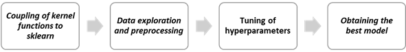
Table 1 Description of the data set.
| Variable | Description | Range | Units |
|---|---|---|---|
| Latitude | Latitude | -8789850.0, -8554950.0 | Meters |
| Longitude | Length | 45000.0, 294750.0 | Meters |
| Band1 | Coastal Band/Aerosol | 0.43,0.45 | Micro meters |
| Band2 | Blue Band | 0.45,0.51 | Micro meters |
| Band3 | Green band | 0.53,0.59 | Micro meters |
| Band4 | Red Band | 0.64,0.67 | Micro meters |
| Band5 | Near Infrared Band NIR | 0.85,0.88 | Micro meters |
| Band6 | Shortwave infrared band SWIR | 1.57,1.85 | Micro meters |
| Band7 | Thermal infrared band | 2.11,2.99 | Micro meters |
| Value | Irradiance | 188.5, 247.3 | 𝑊/𝑚2 |
The geographic coordinates of this dataset are projected in Mercator 3857 as well as the polygon named narino_3857.shp, which was used for geospatial visualization of the predictions. The experiments developed in this study were written using Python language on Google Colab.
B. Coupling Kernel Functions to Sklearn
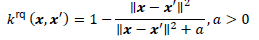
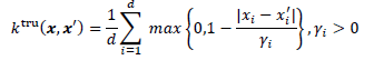
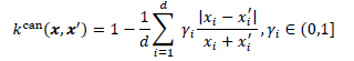
To obtain the best configuration for the SVM algorithm, we initially coupled new kernel functions to it by extending the SVC implementation of the sklearn library for classification as described in more detail in [7], providing the SVM with the rational quadratic, truncated, canberra, radial basic, triangle, and hyperbolic functions. Table 2 shows the mathematical definition of the above kernel functions.
Table 2 Kernel functions coupled to sklearn. Source [2].
| Kernel functions | Formal mathematical definition |
|---|---|
| Rational quadratic (rq) |
|
| Truncated (tru) |
|
| Canberra (can) |
|
| Radial basic (rb) |
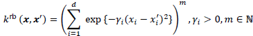
|
| Triangle (tri) |
|
| Hyperbolic (hyp) |

|
C. Data Exploration and Preprocessing
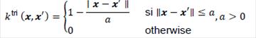
After coupling the kernel functions, the Landsat dataset was loaded and the irradiance (target variable) was converted to a discrete variable, for this purpose 4 different encoders were examined to discretize the variable, namely: equal ranges, k-means, quantiles, and uniform distribution. Figure 2 shows the discretization for 5 classes with the above-described techniques.
As shown in Figure 2., each discretizer offers a different data distribution, although it is advisable to have balanced classes to train a classifier such as the one offered by the discretization in quartiles in this research. We experimented with the 4 distributions, as explained in the next section.
D. Tuning of Hyperparameters
For the comparison of each kernel function to be fair, we experimented using the 4 discretizers of the previous section, 3 different normalizers were used on the feature vector, these are: minimum maximum scaling (MinMax), uniform scaling or standardization (Std), and scaling to the vector norm (Norm). The data was then partitioned leaving 20% of the data for testing, and 80% for training using the 2021 seed (random state). Next, a random search engine was used, configured with a stratified validation with 5 folds. Each search was run on each kernel function (7 kernel functions: 6 from Table 3 plus the RBF function), for each data normalization (3 normalizers) and discretizer (4 discretizers), running a total of 112 searches. The values to be searched for the regularization coefficient (C) are in the logarithmic space with lower bound 0, upper bound 5, consisting of 10 elements. The hyper parameter of each kernel function (coef0 for rational quadratic, gamma for the other kernel functions) is in the logarithmic space with lower bound -4, upper bound 4, consisting of 20 elements.
E. Obtaining the Best Model
Once the hyperparameter tuning was performed, the results were stored to evaluate the commitment of each configuration, in terms of accuracy and training and inference times. Subsequently, the best configurations were chosen for each data discretization and the accuracy of each model was evaluated with the test data. Finally, the extrapolated predictions of this model on all the data were extracted and the geographic visualization was performed, interpolating the data using the Kriging algorithm [9], and the visualization was compared with the maps generated in the state of the art for regression models on these same data.
The following section shows the results obtained.
III. RESULTS
The products generated in this research are shown below. First, the coupling of the kernel functions for classification is shown, followed by the results obtained in the hyperparameter tuning stage, and finally, the maps generated with the best model found are shown.
A. Coupling Kernel Functions for Classification
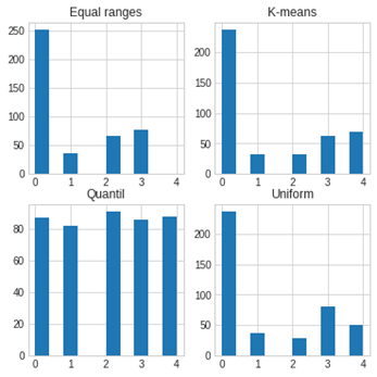
To couple the kernel functions for classification, the SVC class of the Scikit-learn library was extended as shown in Figure 3. There, it is observed that to couple the alternative kernel functions it is necessary to extend the SVC class of Scikit-Learn, once this was done, the constructor of the class was overwritten and the Scikit-Learn Custom Kernel function procedure was used, which transforms the feature vector, using a gram matrix generated from the kernel function defined in the KernelF class. The KernelF class has been implemented by Mora [7].
The above implementation can be installed in Python using the PIP ver command (https://pypi.org/project/sklearnkernels/) and can be contributed to by cloning the following repository (https://github.com/magohector/sklearnkernels).
B. Search Results for Hyperparameter Tuning
As mentioned in the hyperparameter tuning section, several searches were used to perform a fair comparison for each kernel function. For this purpose, 3 pipelines were structured to couple the normalizers and the KSV algorithm. The searches were then run and the results for each discretizer were stored in 3 different CSV files. Table 3 provides a better description of each of the resources obtained.
Table 3 Products obtained in the hyperparameter tuning.
The files listed at Table 3 can be downloaded from the following repository https://github.com/magohector/IrradianceClasiffication. Table 4 shows the consolidated results of the files (.csv) listed, the results with accuracy greater than 0 have been filtered. Table 4 indicating the discretizer (Dis), the normalizer (Sca), the kernel function (kernel), the average accuracy (Mts), the standard deviation of accuracy (Sts), the average training time (Mft), the standard deviation of training time (Sft), the average inference time (Mst), and the standard deviation of inference time (Sst). Table 4 highlights the best results per discretizer and normalizer.
Table 4 Best results obtained in hyperparameters tuning.
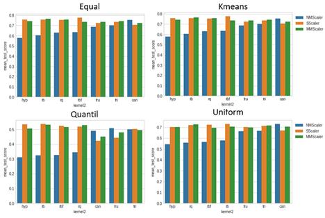
The accuracy of the searches performed in this hyperparameter configuration was also plotted and can be seen in Figure 4, which shows the accuracy (y) axis, kernel function (x) axis (namely: hyp, rb, rq, rbf, tru, tri, and can) and normalizer NMScaler (blue), Sscaler (Orange), NMScaler (Green) for each discretizer.
The best models were taken from each discretizer and the results were evaluated with the test data, where the best configuration obtained an accuracy of 0.8161 for the model with equal discretizer, standard nomalizer, kernel function rbf, gamma equal to 0.000695, and with regularization constant 2154.434690. With this model all the data were extrapolated and interpolated with the ordinary kriging algorithm with a spherical variogram, with a sample of 450 data. Figure 5 shows the data extrapolation, the interpolation of data with classification and the interpolation of state-of-the-art data.
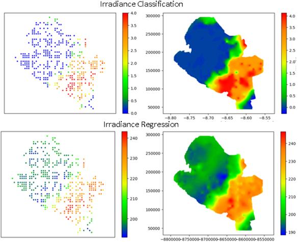
The best models were taken from each discretizer and the results were evaluated with the test data, where the best configuration obtained an accuracy of 0.8161 for the model with equal discretizer, standard nomalizer, kernel function rbf, gamma equal to 0.000695, and with regularization constant 2154.434690. With this model all the data were extrapolated and interpolated with the ordinary kriging algorithm with an Spherical variogram, with a sample of 450 data. Figure 5 shows the data extrapolation (mesh of points) and interpolation for the classification and regression problems, respectively. The same color scale has been used to generate the maps to facilitate visual comparison of the results obtained.
IV. DISCUSSION
As a starting point it is necessary to state that for the purposes of this study the accuracy gain was evaluated for 4 data discretizations, finding that the best way to discretize the irradiance to generate a classification model is the discretizer with equal ranks.
With respect to previous studies focused on the extrapolation of irradiance as a function of the ultraviolet, visible and infrared bands of the electromagnetic spectrum, a new alternative has been proposed, generating the extrapolation from a classification model; however, the accuracy of the model has only reached a value of approximately 0.82, compared to the determination coefficient of 0.94 [7]. Although they are different metrics, it is clear that the regression model has a better-quality metric.
On the other hand regarding the kernel functions in Mora’s regression models [7], it is observed that the standard and min-max normalizers in that order have the best compromise in their quality metrics while in the present study the opposite occurs; min-max and standard.
The present study and that of Mora [7] achieve rbf as the best kernel function in the tuning, the rational quadratic function as the second best kernel function in Mora [7], and radial basic in the present study, all the results in the best normalizer. Regarding the second normalizer, it is observed that the alternative kernel functions gain prominence for both studies, with the min-max normalizer, the rational quadratic, and radial basic kernel functions standing out in Mora [7] as well as in the present study using the standard normalizer.
Finally, when visualizing the extrapolation and interpolation of data in Figure 4, it is observed that the irradiance supply in Nariño has similar segmentation patterns, with more discrepancy in the northern part of the department. However, since there is less variability in the classification model, it is easier to identify the high, medium, and low irradiance zones.
V. CONCLUSIONS
For obtaining classification models applying the SVM algorithm using the Landsat dataset, it is best to use a discretization by equal ranks with standard normalization and with the rbf kernel function, as it has the best compromise in accuracy and time as shown in Figure 3.
The rational quadratic and radial basic alternative kernel functions have a better compromise in accuracy than the rbf function using the max-min normalizer. However, the training and inference time of these functions is longer.
Using the normalizer, the Canberra and Triangular alternative kernel functions excel even in each discretizer, however, the accuracy values are lower than other configurations.
To discretize the irradiance, the best way to obtain irradiance classification models is to use the equal, uniform and kmeans discretizers in that order.

