


Services on Demand
Journal
Article
 English (pdf)
 Article in xml format
 Article references
 Send this article by e-mail
Indicators
-
 Cited by SciELO
 -
 Access statistics
Related links
-
 Cited by Google
 -
 Similars in
SciELO
Similars in
SciELO -
 Similars in Google
Share

 Permalink
Revista de Ciencias
Print version ISSN 0121-1935
rev. cienc. vol.18 no.1 Cali Jan./June 2014
A simple test for asymptotic stability in some dynamical systems
Eduardo Ibargüen Mondragón
Departamento de Matemática y Estadística, Universidad de Nariño, San Juan de Pasto - Colombia
E-mail: edbargun@udenar.edu.co
Miller Cerón Gómez
Departamento de Matemática y Estadística, Universidad de Nariño, San Juan de Pasto - Colombia
E-mail: millercg@udenar.edu.co
Jhoana Patricia Romero Leiton
Instituto de Matemáticas, Universidad de Antioquia, Medellín - Colombia.
E-mail: patirom3@udea.edu.co
Recceived: September 20, 2013
Accepted: November 23, 2013
Abstract
In this paper we analyze asymptotic stability of the dynamical system  =f(x) defined by a C1 function
  is and open set. We ontain a criterion of satabilty for the equilibrium solution
  when the vector field f satisfies
Keywords: ordinary differential equations, asymptotic stability, equilibrium solution.
1. Introduction
In 1982, A.M. Lyapunov developed his stability theory for nonlinear ordinary differential equiations which chaeacterices the behavior of the dinamical systems trajetories in the sense that nearby solutions remain that way from naow on (Hirsch and Smale, (Hirsch & Smale, 1974). .He esablished very useful stabilty criterua for dynamical systems of the form:

The first Lypunow method, also known as Indirect Method of Lyapunov (IML) allows to studying the stability of the equilibrum points for a dynamical system of the type (1) by analyzing the estabilty of the trivial solution for the linearized system:

where G(y) = O(||y||)2. Using the IML, it is possible prove that y = 0 is asymptotically satble if and only if ℌ (λ) < 0 for any eigenvalue λ of the matrix Df(), and so unstable, if there exist an eigenvalue λ of the matrix Df() whit ℌ (λ) > 0. We note that the IML does not allow us to obtain a conclusion if one of the eigenvalues λ of the matrix Df() has a realk part zero, ℌ (λ) = 0 (Khalil, [12]).
In this paper, we will consider the second Lyapunov method, also known as Direct Method of Lyapunov (DML), in which the stability of an equilibrium point requires the fiow associated with the dynamical system (1) being decreased on sorne scalar function V for which is an isolated minimum. This function is known as the Lyapunov function.
For the Lyapunov function V :  where
where  containing the origin, and its orbital derivative
 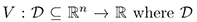 defined by

the DML establishes:
l. If V (x) is positive definite and
(x) is negative semi-definite, then the origin is stable.
2. If V (x) is positive definite and
In general, for any equilibrium solution of (1) the DML states that:
Theorem l. Let  be an equilibrium of (1). Let
  be a continuous function defined on a neigborhood
  differentiable on
  such that
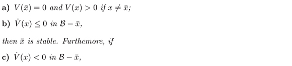
then is asymptotically stable.
In the twentieth century, the DML became in the principal tool to analyze global stability of dynamical systems applied to basic sciences and engineering. The main setback of this method is precisely to find a Lyapunov function, because there is not a systematic method for finding. The suggestion is to propase a function and check if this candidate satisfies the stability conditions (Perko, 1991) .
While the intention of A. M. Lyapunov was to study movement stability (Taylor & Francis, 1992), the DML found a wide range of applications. For example, in problems related with automatic regulation and control of dynamical processes (Rouche et al., 1977; Vasilév, 1981; Yoshizawa, 1966; Artstein, 1978; Barbastin,1970); in competition models (Goh, 1979, 1980; Takeuchi, 1996); in SIR models (Mena-Lorca & Hethcote, 1992; Safi & Garba, 2012); in SIRS models (O'Regan et al., 2010); in models with two compartments (A. Yu, 2003) , and in the proof of the Hopf bifurcation theorem (cited by O'Regan et al., [2010]).
Recently, Lyapunov functions are being applied within the fractional calculus to analyze the stability of dynamical systems. In this field, the method is called Fractional Lyapunov Direct Method (Yan Li et al., 2010; Momani & Hadid, 2004; Zhang et al., 2005; Tarasov, 2007). In 2011, it was used Lyapunov functions to analyze the dynamics of the Hopf bifurcation in a class of models that exhibit Zip bifurcation (Escobar & Gonzáles, 2011, Giesl & Hafstein, 2010, 2012). In 2012 the same authors designed an algorithm to explain the construction of these functions.
There are sorne systems where the Lyapunov function is defined in a natural way, like in the case of electrical or mechanical systems where energy is often a Lyapunov function. In mathematical biology, more precisely in population dynamic modeled through the mass action law, the functions of Goh type

where αi for i= 1,..., n are positive constants that satisfy the first item of Theorem 1 while the other items are reduced to find the constants αi that will satisfy them.
B. S. Goh (Goh, 1979) used the function defined in (2) to prove global stability in mutualism models of the form

In this paper we establish global stability properties for the dynamical system (1) following the same ideas of S. B. Goh in (Goh, 1979). That is, we use the Lyapunov function (2) with specific values of the constants αi to determine the stability conditions.
2. Calculus and linear algebra
Theorem 2. Let E be an open subset of ℝn containing xo, if f : E ⊂ ℝn → ℝ such that f ∈ C3(E), f(x0) = 0 and Hessian matrix Hf (x0) is positive definite, then x0 is a relative minimum of f. Similarly, if Hf(x0) is negative definite, then x0 is a relative maximum of f.
See [15] for proof of Theorem 2.
Theorem 3. (Sylvester's Criterion). A real symmetric matrix is positive definite positive.
See [10] for proof of Theorem 3.
3. Test of stability
In this section we establish a test for the asymptotic stability of the system (1) equilibrium when is an open subset of
 = {(x1,...,xn) ∈ ℝn : xi ≥ 0 for i = 1,...,n}.
 The following proposition relates the equilibrium stability with the sign of certain determinants.
Proposition 1. Let be an open subset of containing  Suppose that the function
  defined in (1) satisfies
  and
and  be the determinants defined by

where aj is a positive constant.
1. IfΔj (
) for j = 1, ... , n are positive, then
1. IfΔj (
Proof. Let a1,...,an be positive constants, for = (x1,...,xn) ∈ , then the function defined in (2) satisfies the condition V() = 0. On the other hand, the i-th term of (2) is:
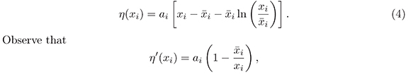
Observe that which implies that η' (xi) > if and only if < xi and η' (xi) < 0 if and only if > xi Thus is a global minimun of η defined in (4). Since η'() = 0, then η'() > 0 for all xi ≠ i therefore V(x) > 0 for al x ≠ . From DML we conclude that if its orbital derivative is negative ( (x) < 0) for all x ∈ / {}, then is asymptotically stable on , while is unstable when (x) > 0 (see Theorem 1).
Observe that (x) = -g(x) where

Since g() = 0 then to prove the stability of it is enough to verify that is a minimum of g on , and any other equilibrium solution y ∈ of (1) satisfies that g(y) ≥ g(). The derivative of g is given by the gradient vector
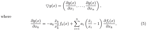
for k = 1,...,n. From (5) we have that ∂g()/∂xk = 0 for k = 1,...,n, which implies ∇g() = 0. Therefore is a critical point of g.
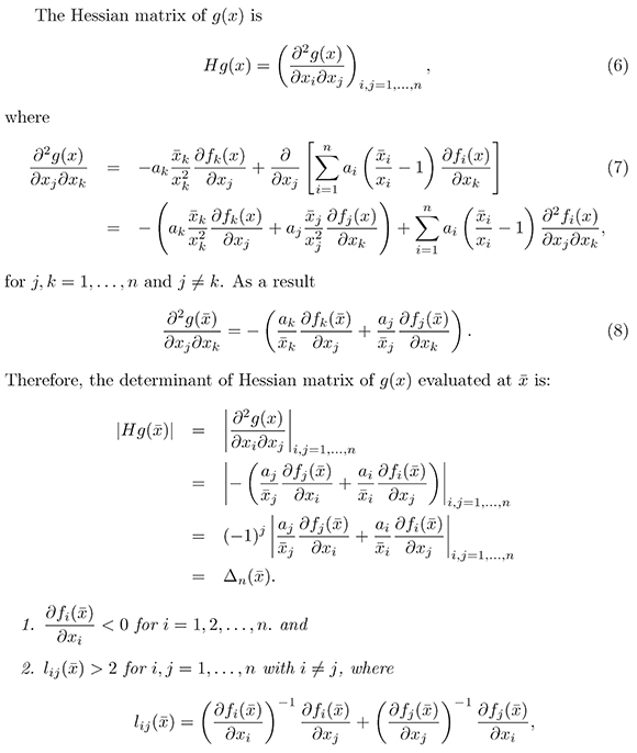
Since Hg() is a symmetric matrix, and assuming that all its principal minors are positive, then from Theorem 3 we have that is a local minimum of g on . Now, suppose that y ∈ is another equilibrium solution of (1) then g(y) = g() = 0. Similarly it is verified that if its principal minors have alternating signs for k = 1,...,n, starting with a negative value, then is unstable, which completes the proof.
From the above proposition, the following corollary is derived:
Corollary 4. If the Hessian matrix Hg(x) defined in (6) evaluated at is positive definite, then is globally asymptotically stable on and unstable when Hg() is negative definite.
The following theorem summarizes the main result of this work. The novelty of next test consists in replacing the expertise of the authors to find the constants ai defined in (2) for conditions easy to verify.
Theorem 5 (Stability Test). Let  be an equilibrium solution of nonlinear system ( 1). If
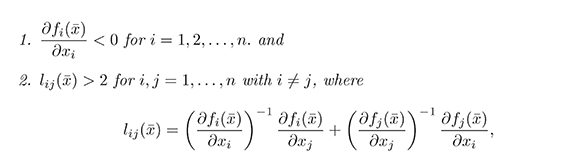
then is globally asymptotically stable.
In consequence, from Corollary 4 we conclude that is globally asymnt.nt.irallv stable in .
4. Application of main result
4.1 Numerical solutions
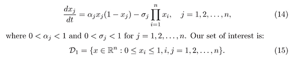
In this section we will apply the Theorem 5 to prove the asymptotic stability of nontrivial equilibrium of the nonlinear system
The following lemma ensures that all solutions of (14) starting in The following lemma ensures that all solutions of (14) starting in t ≤ 0
Lemma 6. The set 1 defined in (15) is positively invariant for the solutions of the system (14).
Proof. Let x (x01, x02,...,x0n) be given. If there is 1 ≤ j ≤ n such that x0j = 0 then we see directly from the unique and existent result that xj(t) ≡ 0 for all t ≥ 0, and so for k ≠ j such x0k ≠ 0, we have that xk(t) satisfies the logic differential equation:

for which we know that 0 ≤ xk(t) ≤ 1. In other words, if there is 1 ≤ j ≤ n such that x0j = 0, we have that 0 ≤ xk(t) ≤ 1 for 1 ≤ k ≤ n. Now, we assume that x (x01, x02,...,x0n) ∈ 1 is such that x0j ≠ 0 for any 1 ≤ j ≤ n In this case, we know that xj(t) for any ≤ 0 and 0 ≤ j ≤ n. Then, from (14) we obtain:

or equivalently

Let z = x-1j, then dz/dt = -x-2jdxj/dj. Substituting z and dz/dt in (16) we have

Multiplying the above inequality by eαjt we obtain:

Integrating the inequality (17) between O and t we have:

Substituting z = x-1j in (18) we obtain:

Therefore, we conclude that:
O ≤ xj(t) ≤ 1 for all t ≤ O.
maening x = (x01, x02,...,x0n) ∈ 1 as desired
The next proposition summarizes existent results of the equilibrium solutions of (14).
Proposition 2. The system (14) has at least 2n+1 -1 equilibrium solution in 1
Proof. The equilibrium solutions of (14) are given by the solutions of the algebraic system

Observe that in the following cases, a)xj = 0, b)xj = 1 and xk = 0 for j ≠ k, the equations (19) are satisfied, which implies the existence of 2n - 1 equilibrium of the form x0 = (p1,...,pn) where pj = 0 or pj = 1.
One of the possible applications for system (14) when n = 3 could be the On the other hand, from (19) we obtain:
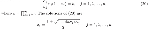
The above implies that xj > O if and only if O < k < αn/4σn. Therefore, there are at least two equilibriums in int (1). This completes the proof.
The following proposition summarizes stability results of the equilibrium of(14).
Proposition 3. Suppose that the system (14) has an interior steady state ∈ 2 ⊂ 1 where
2 = {x ∈ ℝn : 0 ≤ xi ≤ 1,0 ≤ xi + xj, ≤ i j = 1,2,...,n}.
then this steady state is globally asymptotically stable on the interior set of 1.
Proof. From (14) we conclude that:
From hypothesis ∈ 2, results that 0 < 1 + j < 1 which implies (i + j)2 < i + j, or equivalently (1-i) + (1-)j > 2ij. The above implies that the second hypothesis of Theorem 5 is satisfied. That is lij > 2. Therefore is globally asymptotically stable on interior set of 1.
4.1. Numerical solutions
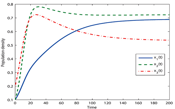
One of the possible applications for system (14) when n = 3 could be the competition among three species with logistic growth. The simulation of Figure 1 was made with the following data: α1 = 0.1, α2= 0.2, α3= 0.15, σ1 = 0.08, σ2= 0.15 and σ3= 0.14. In this case the solutions of (14) tend to the coexistent equilibrium P1= (0.68,0.72,0.53) which agrees with the theoretical results.
Figure 1.Graphs of the component solutions x1, x2 and x3 of (14) for n = 3. In this case, α1=0.1, α2=0.2, α3=0.15, σ1=0.08, σ2=0.15, σ3=0.14.
5. Conclusion
In certain areas of applied mathematics such as Biomathematics, the qualitative analysis of the solutions of dynamical systems defined by ordinary differential equations is fundamental to understand problems in biology (Ibargüen et al., 2011). In this sense, the DML is very practical and widely used to analyze the stability of dynamical systems. In this article we use the DML to establish easier conditions to verify the assurance of global asymptotic stability of the equilibrium solutions of some dynamical systems. The fact that these conditions are defined in terms of  suggest the possibility that the stability test (Theorem 5) can be used to numerically verify asymptotic stability.
Acknowledgements
We want to thank to anonymous referees and Dr. L. Esteva for their valuable comments and suggestions that helped us to improve the paper. E. Ibarguen acknowledges support from project No 082-16/08/2013 (VIPRI-UDENAR).
References
Alexandrov, A. Y. (2003). On the Construction of Lyapunov Functions for Nolinear System. Differential Equations, 41 (3), 303-309. [ Links ]
Artstein, Z. (1978). Uniform Asymptotic Stability via the Limiting Equations. J. Diff. Equat., 27 (2), 172-189. [ Links ]
Barbashin, E. A. (1970). Lyapunov Functions. Nauka, Moscow. [ Links ]
Escobar, C., y Gonzáles, J. (2011). Dinámica de la bifurcación de Hopf en una clase de modelos de competencia que exhiben la bifurcación Zip. Revista de Ingeniería Universidad de Medellín, 10 (19), 159-169. [ Links ]
Giesl, P., & Hafstein, S. (2010). Existence of Piecewise Affine Lyapunov Functions in two Dimensions. J. Math. Anal. Appl., 371 (1), 233-248. [ Links ]
Giesl, P., y Hafstein, S. (2012). Construction of Lyapunov Functions for Nonlinear Planar Systems by Linear Programming. Journal of Mathematical Analysis and Applications, 388 (1), 463-479. [ Links ]
Goh, B. S. (1979). Stability in Models of Mutualism, The American Naturalist. The American Society of Naturalists, 113 (2) 261-275. [ Links ]
Goh, B. S. (1980). Management and Analysis of Biological Populations. Amsterdam, Netherlands: Elsevier Science. [ Links ]
Hirsch, M., & Smale, S. (1974). Differential Equations-Dynamical Systems and Linear Algebra. New York, USA: Academic Press. [ Links ]
Hoffman, K., & Kunze, R. (1971). Linear Algebra (2 ed.). Englewood Cliffs (NJ), USA: Prentice-Hall. [ Links ]
Ibargüen-Mondragón, E., Esteva, L., & Chávez-Galán, L., (2011). A Mathematical Model for Cellular Immunology of tuberculosis. Journal of Mathematical Biosciences and Engineering, 8 (4), 973-986. [ Links ]
Khalil, H. (1996). Nolinear System (2 ed.). London, UK: Prentice-Hall. [ Links ]
Li, Y., Chen, Y., & Podlubny, I. (2010). Stability of Fractional-order Nonlinear Dynamic Systems: Lyapunov Direct Method and Generalized Mittag-Leffler Stability. Computers and Mathematics with Applications, 59 (5), 1810-1821. [ Links ]
Lyapunov, A. M. (1992). The General Problem of the Stability of Motion. London, UK: Taylor and Francis. [ Links ]
Marsden, J., & Tromba, A. (1976). Vector Calculus. New York, USA: W. H. Freeman and Company. [ Links ]
Mena-Lorca, J., & Hethcote, H. W. (1992). Dynamics Model of Infectious Diseases as Regulator of Populations Sizes. J. Math Biol, 30, 693-716. [ Links ]
Momani, S., & Hadid, S. (2004). Lyapunov Stability Solutions of Fractional Integer-differential Equations. International Journals of Mathematics and Mathematical Sciences, (47), 2503-2507. [ Links ]
O'Regan, S. M., Kelly, T. C., Korobeinikov, A., O'Callaghan, M. J., & Pokrovskii, A. V. (2010). Lyapunov functions for SIR and SIRS epidemic models. Applied mathematics letters, 23 (4), 446-448. [ Links ]
Ogata, K. (1990). Moderm Control Engineering (2 ed.). London, UK: Prentice-Hall. [ Links ]
Perko, L. (1991). Differential Equations and Dynamical Systems. New York, USA: Springer. [ Links ]
Rouche, N., Habets, P., & Laloy, M. (1977). Stability Theory by Liapunov's Direct Method. New York, USA: Springer-Verlag. [ Links ]
Safi, M. A., & Garba, S. (2012). Global Stability Analysis of SEIR Model with Holling Type II Incidence Function; Computational and Mathematical Methods in Medicine. New York, USA: Hindawi Publishing Corporation. [ Links ]
Takeuchy, Y. (1996). Global Dynamical Properties of Lotka-Volterra System. Singapore, Singapore: World Scientific. [ Links ]
Tarasov, V. E. (2007). Fractional Stability. Recovered 15/10/2016 http://arxiv.org/abs/0711.2117v1 [ Links ]
Vasilév, S. N. (1981). The Comparison Method in the Mathematical Theory of Systems. Uravneniya, 17 (9), 1562-1573. [ Links ]
Yoshizawa, T. (1966). Stability theory by Liapunov's second method, (v. 9). Tokyo, Japan: Mathematical Society of Japan. [ Links ]
Zhang, L., Li, J., & Chen, G. (2005). Extension of Lyapunov Second Method by Fractional calculus. Pure and Applied mathematics, 3, 1008-5313. [ Links ]

Revista de Ciencias por Universidad del Valle se encuentra bajo una licencia Creative Commons Reconocimiento 4.0.

