


 English (pdf)
 Article in xml format
 Article references
 Send this article by e-mail
 Cited by SciELO
  Cited by Google
  Similars in
SciELO
Similars in
SciELO  Similars in Google
 Permalink
INTRODUCTION
Rice is of great importance for Colombia because it is the second largest rice producer in Latin America and the Caribbean. Rice occupies the first place in terms of economic value among short-cycle crops and is the primary source of calories and protein for the low-income group; which accounts for about 20% of the country’s population. The national average per capita rice consumption in 2000 was 45.3 kg of brown rice. In addition to local production, Colombia even has to import additional rice to meet demand.
Rice is an important food source which should be at low moisture content for safe storage. Unfortunately, the moisture content of rough rice after harvesting is about 24% dry basis, which encourages the growth of molds (1). In order to conserve the rice in a proper way the moisture content has to be near 14% dry basis (2). A topic of economic importance related to the drying process is the cracking of the rice kernel. Larger grains are more expensive than smaller grains, so it is important to prevent cracking. This can only be done if the drying process is carried out in stages with a certain temperature and air velocity. Another factor that limits the maximum temperature is the degradation of the quality of the grain due to increased enzymatic inactivation (1). Because of the sensitivity of the rice and since rice drying is an energy-intensive process; increasing the efficiency of the drying process has important economic consequences for both rice producers and for consumers.
A simple model with a simultaneous heat and mass transfer during rice drying in a deep-bed was developed in (3). The drying process can be divided into three different stages: Dynamic drying, fixed bed drying and removing the internal stress, we focus on the Fixed bed drying part of the process which can be approximated by a curve like in Figure 1(4); as rice is a hygroscopic material.
Physical models
In order to understand the drying process physically, it is necessary to see how the moisture content is evolving in time inside the plenum as well as inside the rice kernel. To accomplish this plenum is divided in thin layers which are consisting of single rice kernels.
The rice kernel on its own is a very complex biological grain, so a simplification has to be made. The grain is taken as a non-axially symmetrical ellipsoid divided into three layers: hull, bran and endosperm. The drying process itself is dominated by convective heat and mass transfer, so neglecting of conduction does not result in a significant error. Based on the above assumptions, the three-dimensional governing equations [1, 2] in a Cartesian coordinate system can be expressed as:
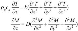 (1)
(1)
Boundary conditions:
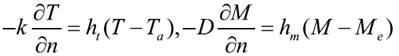 (2)
(2)
Where,
T is temperature in °C; M is the moisture content in % dry basis [d.b]; D is the diffusion coefficient in m2s-1; k is the thermal conductivity in W m-1 °C-1; ( is the time in s;(g is the kernel density in kgm-3;cg is the rice specific heat capacity in J kg-1°C-1.
Initial conditions: when (=0,
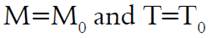
To get a numerical solution to this partial differential equation (second order linear partial differential equation) that is close to the real solution, it is necessary to have an accurate numerical representation of the boundary conditions.
To solve the PDE it is necessary to specify the initial and boundary conditions. Between the existing numerical methods, probably the most used in the PDE solution is the method of finite differences. In this kind of problems, the solution moves forward indefinitely from known initial values, always satisfying the boundary conditions. The basic concept of the method is relatively simple, but the implementation is often complex (5). The procedure is to discretize the domain of integration of the PDE by using a mesh discretizing the PDE and its conditions, obtaining algebraic equations for each node (such nodal equations are related in a way that a system of equations algebraic is obtained), and finally write a program to solve the system of algebraic equations. Algebraic system solution represents the values of the PDE solution.
Many researchers have modeled thin layer drying using Fick’s law or empirically desire equations (6). In the works of (7-10) appear results on computer base grain drying control systems. Although these models provide fast data acquisition during complex experimental conditions and versatility of operations through software control, they presented several implementation complexities.
In (11) four thin-layer equations were derived by regression analysis to predict the drying behavior for deep-bed drying of rough rice. The effects of drying air temperature, drying air absolute humidity, drying time interval, and tempering time interval were considered.
These mathematical models presented several complexities which increase the computational cost. On another hand they use several approximations that decrease the performance of the models. Hence, if they must be used in combination with model-based control strategies, faster and more accurate models have to be used. That is why nonlinear models based on artificial neural networks are explored.
In this paper supervised neural network topologies was used. Artificial neural networks (AANs) were used for the prediction of equilibrium moisture content of three varieties of paddy (Caribe -8, Orizica -1, Yacu -9), (12), Authors used to feed forward back-propagation and cascade forward backpropagation networks with Levenberg-Marquardt and Bayesian regularization training algorithms to train the input data patterns.
The algorithm was developed using Matlab/Simulink, some related information can be found in (13, 14). In (15) a feed-forward neural network topology is presented to model the non-linear drying process and it uses a multilayer perceptron for modeling the drying of the production of a coconut process and in (16) modeling and control of drying process using neural networks is presented.
Dynamic Neural Networks
Unlike the feedforward network, where there is an algebraic relationship between input and output, this architecture contains memory. There is feedback on the output and the inputs have a certain delay. The basic equation of the network is:
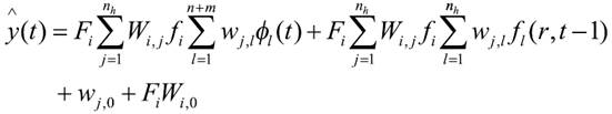 (3)
(3)
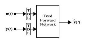
In Figure 1 the topology of a dynamic neural network is presented (14). A Narx topology of the dynamic neural network is presented in this paper. There are two different versions of Narx topologies. The parallel architecture feeds the predicted output signal back to the input latter. The series-parallel architecture uses the measured output signal as input. The latter will be used for the following reasons: a) The input to the feedforward architecture is more accurate because it is the real measured output signal, and b) A second advantage is that the resulting network has a pure feedforward architecture, which allows static backpropagation to train it.
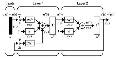
A general way of looking at the efficiency of embedding a problem in a neural network comes from a computational complexity point of view. Solving a problem on a sequential computer requires a certain number of steps (times complexity), a certain memory size (space complexity), and a certain length of the algorithm. The several topologies of the neural NARX neural networks can be seen in Figures 1 and 2 (14).
In (17) the kinetics of convective deep-bed drying of rough rice using NN to study the energy performance of the process is presented. (18) an optimal multi-layered, feed-forward, artificial neural network (MLFF-ANN) model for predicting the moisture ratio of paddy during the drying process was investigated.
MATERIALS AND METHODS
Physical Plant
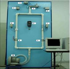
There is a scale model of the fixed bed inclined floor dryer. In the inclined floor furnace, hot air, generated by a fan and a heating resistance, is blowing from under the rice upwards through the plenum. In order to model and control the process, there are two thermocouples to measure the temperature of the rice, another one to control the air temperature and a moisture content sensor to determine the humidity of the rice. The airflow and the air temperature are the parameters that can be adapted to control the process, but in industrial applications only the air temperature is variable. The temperature is adapted by a Pulse Width Modulated resistance regulated by a PID controller with integrated anti-windup to prevent accumulation of the integration error which is caused by the slow temperature time constant. The air flow can be regulated by a frequency modulated scalar control. Measurements are collected by a Labview-program, but the model and the control of the drying process are implemented in Matlab. To carry out the experiments a thin layer dryer was tested. Figure 3 shows the prototype of the system to identify:
1) Pressure meter transformer; 2) Heating resistance; 3) Electrical transformer; 4) Electric circuit of the resistance; 5) Electronic controller of the plant; 6) Differential pressure meter; 7) Differential pressure meter; 8) Pneumatic valve; 9) Pneumatic valve; 10) Fan.
Experimental setup
To identify the nonlinear system, some signals have to be selected. The following signals were chosen for this purpose.
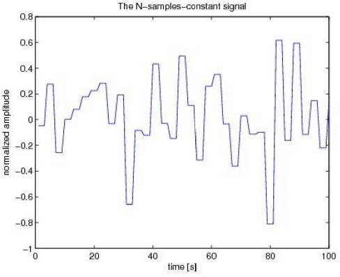
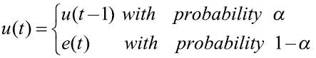
If e (t) is a white noise signal; the N-sample-constant signal (Figure 4) is defined by:
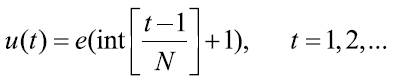 (4)
(4)
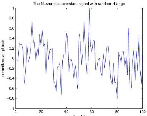
This is an extension to the N-samples-constant. Another random variable (Not a predefined integer) will decide when to change the level of the input signal (Figure 5).
 (5)
(5)
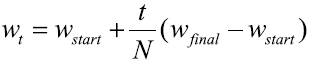
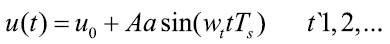
A chirp signal is a signal in which the frequency increases with time (Figure 6). With
his signal, it is possible to excite the desired frequency range. When applying this signal to a nonlinear system, different DC- values, and amplitudes have to be taken.
 (6)
(6)
 (7)
(7)
The bandwidth is a representation of the response time of the system. Experiments were conducted at two drying air temperatures and the airspeed remained at a constant level because it is shown that air velocity only has a very weak dependence of moisture ratio. In order to get this response time, the following test is performed: Test 1 (Air temperature: 40°C, 7 hours), Test 2 (Air temperature: 35°C, 33 hours).
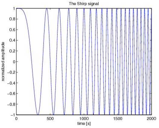
At the transition, there is a transient that is characterizing the bandwidth. To determine the length of this transient a curve fitting was performed as can be seen in Figure 7. The fitted curves and the filtered version of the original test data are compared. Clearly, the transient is approximately 2.5 hours. As a linear approximation of the system a first-order dynamic is proposed:  , where 1/τ corresponds to the bandwidth. The rule of Thumb says that the reaction time of the system (2.5 h) is five times, such that the bandwidth equals 1/1800 Hz.
RESULTS AND DISCUSSION
In this section, the results for the feed forward back-propagation and the dynamic neural networks topologies are presented.
Feed Forward Back-Propagation Neural Network
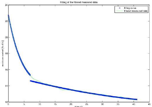
In Figure 8 the response of the feedforward back-propagation neural network to validation data is compared with the original data. As can be seen, the results follow some of the dynamics of the system, however, the predictive curve is totally out of the range of the real data.
Dynamic Neural Network
In Figure 9 the response of the Dynamic Neural Network to validation data is compared to the original data. As can be seen, the result follows almost perfectly the dynamics of the process. In Figure 10 the error between the predicted and the real values of the moisture are presented.
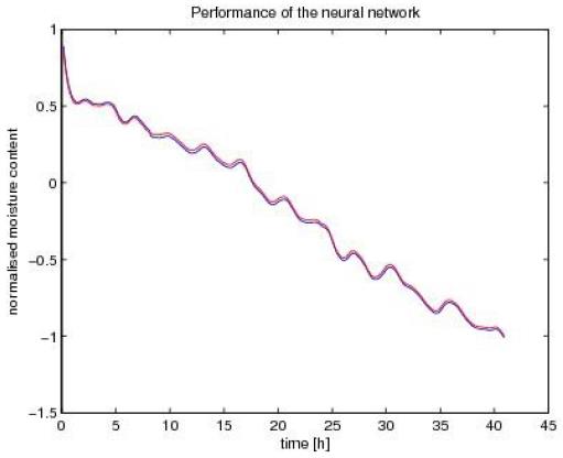
Figure 9 Validation data (red) vs real data (blue) from a test experiment using dynamic neural networks topology.
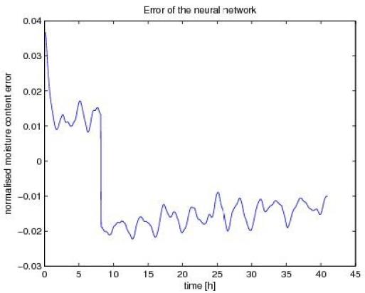
Figure 10 Error between predicted and real values in a test experiment using a dynamic neural network.
When generating a new neural network using datasets for training, the result of the network always has to be checked, because they are non-deterministic, so sometimes the result after the training can be very bad; the network is useless and training has to be done again. A network with a lot of layers does not especialy gives the best result. A short network has the advantage of needing less training computations. Optimizing all the network parameters is a time consuming task; everytime a parameter is changed, the network has to be trained again. In general, it can be said that the approximations done by the networks to obtain a nonlinear model of the rice drying process are quiet good. They can be a lot better if more datasets for training are available.
Sometimes the training of the network stops before a good network appears, the reinitialization and training of the network must be done again. In general, the biggest problem of the project realization is the little available data for training and simulating the network. Using big networks with a lot of layers results in a lot of calculations, this is also an important factor that has to be taken into account. It can also be concluded that when some parts are given as training, even with one dataset, a back-propagation network simulates very well the other parts of the drying curve. Advantages of this strategy can be seen in (19), where an independent multilayer neural network approach was used to predict the performance of the dryer for drying of rice, and in (20), where by applying the artificial neural networks (ANNs), moisture content of paddy was predicted under the various input conditions.
CONCLUSIONS
This paper presents an application of artificial neural network (ANN) technique to develop a model representing the non-linear drying process. The air heat plant (AHP), an important component in drying process is fabricated and used for building the ANN model. An optimal feed forward neural network topology is identified for the air heating system set-up. The training sets are obtained from experimental data. Back-propogation algorithm with momentum factor is used for training. The results show that the back-propogation ANN can learn the functional mapping between input and output. The advantages of ANN model developed for AHP is highlighted. The developed model can be used for control purposes.
The neural networks are suitable for modeling nonlinear systems. However, some things have to be taken into account; the training data have to be selected in such a way that all the information related to the dynamic of the process is presented; the number of layers and the kind of activation function has to be selected in a proper manner, in order to obtain the best configuration as possible. Some topologies include also grain temperature for better performance.
On another hand, the characteristics of the process will lead us to the selection of a topology of the neural network. In this work, the memory present in the drying process affects the performance of the simple feed forward back-propagation neural network. The dynamic neural network, on the contrary, feeds the output of the system, has the capacity to act based not only in the present data but also on the past input and outputs. For this reason, the performance of the dynamic NN is much better compared with the other topology.

