


Servicios Personalizados
Revista
Articulo
 Inglés (pdf)
 Articulo en XML
 Referencias del artículo
 Enviar articulo por email
Indicadores
-
 Citado por SciELO
 -
 Accesos
Links relacionados
-
 Citado por Google
 -
 Similares en
SciELO
Similares en
SciELO -
 Similares en Google
Compartir

 Permalink
Suma Psicológica
versión impresa ISSN 0121-4381
Suma Psicol. v.17 n.1 Bogotá ene./jun. 2010
Within-Session Analysis of the Extinction of Pavlovian Fear-Conditioning Using Robust Regression
Análisis intra-sesión de la extinción del condicionamiento pavloviano de miedo usando regresión robusta
* Virginia Commonwealth University, Estados Unidos
** Fundación Universitaria Konrad Lorenz, Bogotá, Colombia. Author note: This research was partially funded by a grant from the A.D. Williams Foundation to the second author.
Correspondence should be sent to, Cristina Vargas-Irwin, Fundación Universitaria Konrad Lorenz, Carrera 9 bis N. 63-42, Bogotá, Colombia, Tel: (571) 3472311 Ext. 111, Fax: (571) 3472311 Ext. 131, e-mail: cvargas@fukl.edu
Recibido: Julio 26 2010 Aceptado: Agosto 26 2010
ABSTRACT
Traditionally, the analysis of extinction data in fear conditioning experiments has involved the use of standard linear models, mostly ANOVA of between-group differences of subjects that have undergone different extinction protocols, pharmacological manipulations or some other treatment. Although some studies report individual differences in quantities such as suppression rates or freezing percentages, these differences are not included in the statistical modeling. Withinsubject response patterns are then averaged using coarse-grain time windows which can overlook these individual performance dynamics. Here we illustrate an alternative analytical procedure consisting of 2 steps: the estimation of a trend for within-session data and analysis of group differences in trend as main outcome. This procedure is tested on real fear-conditioning extinction data, comparing trend estimates via Ordinary Least Squares (OLS) and robust Least Median of Squares (LMS) regression estimates, as well as comparing between-group differences and analyzing mean freezing percentage versus LMS slopes as outcomes.
Keywords: fear conditioning extinction, within-session dynamics, robust regression, linear models, Least Median of Squares.
RESUMEN
El análisis de datos de extinción en experimentos de miedo condicionado ha involucrado, tradicionalmente, el uso de modelos lineales estándar, primordialmente ANOVA de diferencias entre grupos de sujetos sometidos a diferentes protocolos de extinción, manipulaciones farmacológicas o algún otro tratamiento. Aún cuando algunos estudios reportan diferencias individuales en indicadores como tasas de supresión o porcentajes de congelamiento, esas diferencias no son incluidas en el análisis estadístico. Los patrones de respuesta intrasujeto son entonces promediados usando ventanas temporales de baja resolución, las cuales pueden ignorar esta dinámica del desempeño individual. Este trabajo ilustra un procedimiento analítico alternativo que consta de 2 pasos: estimación de la tendencia para los datos intrasesión y el análisis de las diferencias entre-grupo usando la tendencia como variable de respuesta. Este procedimiento se pone a prueba usando datos reales de extinción de miedo condicionado, comparando estimaciones de tendencia robusta vía Mínimos Cuadrados Medianos con Mínimos Cuadrados Ordinarios, y comparando las diferencias de grupo usando la pendiente robusta versus la mediana del porcentaje de congelamiento como variable dependiente.
Palabras clave: extinción del miedo condicionado, dinámica intra-sesión, regresión robusta, modelos lineales, Mínimos Cuadrados Medianos.
Contemporary research in Pavlovian conditioning has usually involved the use of group comparisons, and considerable attention has been given to its appropriate control procedures, with Rescorla’s classical paper on this subject totaling over 740 citations in the 43 years since its publication (Rescorla, 1967). Analysis of extinction data in fear conditioning experiment has followed this general methodological pattern: traditionally, it involves the use of standard linear models, mostly ANOVA of betweengroup differences of subjects that have undergone different extinction protocols, pharmacological manipulations or some other treatment. Although some studies report individual differences in quantities such as suppression rates or freezing percentages, these differences are not included in the statistical modeling. This between-subject approach in data analysis contrasts sharply with theoretical treatments of Pavlovian conditioning, which usually model associative changes through time (Mackintosh, 1975; Pearce & Hall, 1980; Rescorla, 1997; Rescorla & Wagner, 1972). What is more, many core assumptions of computational models refer to temporal dynamics of within-subject data, such as the negative acceleration of both acquisition and extinction (Killeen, Sanabria & Dolgov, 2009; Rescorla, 2001). Averaging within- subject patterns using coarse-grain time windows can overlook these individual performance dynamics.
There are several approaches to incorporate within-session dynamics information into the analysis. Complex modeling frameworks such as growth-curve models and Mixed-Effects Linear Models (MLM) could be considered. However, as an improvement to the conventional mean-difference analysis, a simpler two-step linear modeling strategy is proposed.
In the first step individual dynamics are summarized as a linear trend slope, which is then treated as a dependent variable in between- group analysis. Similar procedures are well-known and widely used in several fields, especially in econometrics, however its application to extinction data, and in particular to fear-conditioning experiments is rather unusual (Adichie, 1975; Sen, 1972; Tabatabai & Tan, 1985). This paper intends to illustrate the application of the 2-step modeling procedure to the specific preparation of fear-conditioning extinction, using real data from a group experiment.
The first step requires the summarization of the within-subject data into a single parameter. For this critical operation, a robust regression method is proposed as the key component of the analysis. Visualization of individual within- session extinction curves is combined with the robust regression procedure as a more complete approach to individual dynamics. The application is outlined avoiding excessive statistical complexity, with the model specification details and the results and interpretation are discussed to help behavioral researchers to take advantage of this procedure for their own experimental data.
While there are limitations in any analytic technique, and specific considerations in each experiment that most general statistical techniques won’t solve automatically, the tradition of presenting statistical results for fear-conditioning data, and the expectation from most journals that experimental outcomes be interpreted at least in part, based upon statistical results, leads to a situation in which a more appropriate statistical technique is needed.
Current statistical practices in the analysis of extinction
Several fear conditioning extinction studies report linear models results. Generally, one-way (single-level) ANOVA analysis or t-tests are performed and reported (Brooks, Vaughn, Freeman & Woods, 2004; Rescorla, 2006). The statistical tests focus on the mean differences between groups at the end of the extinction phase.
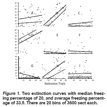
Although some studies show graphical displays of within-subject dynamics, such level of analysis is seldom treated statistically. To illustrate the limitations of global session average as an indicator of the extinction process, we illustrate how two extinction curves with very different features can have the same average. Figure 1 shows two hypothetical extinction curves (sampled from within-session data): estimating the average or the median for the session would render both subjects performance identical. While S2 shows a cyclic pattern with strong late spontaneous recovery, S1 shows a step and steady initial decline with moderate late spontaneous recovery. The features of both curves establish strong differences in extinction; however, the analysis of average performance would yield the conclusion that both processes are exactly the same. Without resorting to more complicated non-linear or multi-parameter models, by simply taking the linear trend, the slope for S2 is 3.93 larger than S1 slope. While the mean, median or session total, are economical ways to represent the session performance, it is clear the linear slope (which also constitutes a single quantitative indicator) seems to be more sensitive to differences in the extinction curves.
The use of extinction slopes is especially important given the current emphasis in the pharmacology of extinction (Myers & Davis, 2007): drugs such as NMDA agonists, for example, are thought to enhance extinction(Ledgerwood, Richardson & Cranney, 2004; Richardson, Ledgerwood & Cranney, 2004), and separating pharmacological effects on extinction from effects on conditioning has proved to be one important challenge in this field. Endpoint measures of extinction confound initial conditioning levels and extinction rates, while difference scores or the use of initial conditioning levels as covariates also provide inadequate estimation of extinction rates. Even repeated measure ANOVAS of extinction data are obscure in differentiating initial conditioning levels and extinction rates. Extinction slopes, on the other hand, provide a straight forward index of the speed of extinction.
The usual data structure resulting from a fear conditioning experiment includes the following components:
-
An individual time series of responses (i.e. movement index, freezing percentages), indexed by time units or trial discrete indexes.
-
Session totals, averages or global indicators, which can become a series in a multisession experiment.
-
 Group-totals, aggregated values for response indicators, pooled for each group In general, only group totals are analyzed and individual within-session dynamics are not modeled. Conventional ANOVAs using global quantities as outcomes, for instance suppression ratios, ignore individual dynamics, and collapse all data into group information. It is difficult to argue against representing session data with a single quantity, given the elegance of this representation and the parsimonious analysis it allows. Trying to use complex models representing most of the features of individual within-session curves, may lead to multiple parameters per session, losing the simplicity of conventional group-difference analysis for a single quantity.
However, this single quantity can be chosen to be more sensitive to the features of the dynamics of fear response extinction. Part of the proposed 2-step procedure involves choosing the representation of within-session data.
Data analysis in 2 steps
The 2 steps involved in the proposed procedure are simple enough to be compatible with the current practices in data analysis for fear conditioning experiments.
Step 1. Estimate a trend for within-session data. Step 2. Analyze group differences in trend as main outcome. There are several ways to perform these steps. The proposed procedure can be detailed as follows:
Step 1. Within-session analysis. This step is aimed to obtain a single quantity representing session data, which can then be used to compare groups and estimate treatment effects. The purpose of this step is not to estimate effect sizes or make statistical inferences.
Individual (within-subject) time series can analyzed according to the following model:
Y = a + bT
Where Y is the individual time series of fear responses (i.e. freezing percentage) for a single subject, a is the intercept, T is a within-subject level predictor, in this case a linear polynomial of discrete time units (i.e. extinction trials), and b is a parameter representing the effect of time T (slope). The parameter b represents the rate of change in the within-subject response over time, and can be considered as an estimation of extinction rate. This model states that the within-subject time series depends on an initial level (conditioning level) and a trend (slope or rate of extinction).
More complex models could be specified, including non-linear or auto-regressive processes (McAleer, Chan, Hoti & Lieberman, 2008). However, a linear trend is considered a substantial improvement over the sum, mean or median of the series, while retaining relative simplicity of interpretation for the fear-conditioning researcher. On the other hand, the linear trend targets one of the key features of an extinction curve: expected steep decline in fear response over time. Extinction data may include several bins or data points (i.e. 20-40), which implies that using a single parameter would be parsimonious representation. A complex model may require several parameters to represent 20 data points, which is not practical from a data-analysis perspective.
Within the simplicity of the linear trend, there are subtle differences in procedure. Ordinary Least Squares (OLS) regression is the ubiquitous procedure for estimating linear trends. However, for the particular application to fear conditioning extinction, OLS suffers from a key weakness which is sensitivity to extreme values. This means that a spontaneous recovery feature, with a peak freezing response value late in the session, can greatly affect the b parameter as estimated by OLS, resulting in global decline trends “flattened” or compensated by late peak values. To overcome these issues, a robust regression procedure can be employed.
Robust regression procedure: Least Median of Squares. A robust regression procedure to estimate b may be more appropriate, not only because of its resistance to extreme values, but also because of the limited number of time points (or bins) used to analyze some withinsession series. It is possible to analyze these series using high-resolution data (Vargas-Irwin & Robles, 2009), however the procedure should apply to medium-low resolution data as well.
There are several robust procedures for estimating linear trends, each one with different properties. From those procedures, a method called Least Median of Squares (LMS, Rousseeuw, 1984), is robust enough for the goals of Step 1, and it is well-known and relatively easy to interpret. In simple terms, instead of minimizing the sum of square errors, LMS minimizes the median of square errors. Given a vector of observed values Y, and a vector of predicted values Y’, OLS regression estimate parameters minimizing the quantity sum(e2), while LMS minimizes Median(e2), where e is the residual term, defined as Y-Y’.
In general, if fear response peaks appear late in the session, or if erratic points across the series amount less 50% of the within-session data points, LMS estimation of b will be unaffected. This is what is technically called the breakdown point of a robust estimate (Hampel, 1971). LMS estimates have what is considered a high breakdown point, up to 50%, and have other interesting properties regarding scales and transformations, which makes them useful for a wide variety of applications (Mount, Netanyahu, Romanik, Silverman & Wu, 2007).
There are alternative procedures to LMS (Hubert, Rousseeuw & Van Aelst, 2008; Ludbrook, 2010), and there may be limitations in terms of the quality of LMS estimators from a statistical inference standpoint or in terms of algorithm optimality. However, in its original formulation, LMS was intended as a data analysis procedure, instead of an optimal parameter estimation technique (Rousseeuw, 1984, p. 873). Fear response extinction trends are employed here to accomplish a data analysis goal, rather than statistical inference. The interest here is to capture a key feature of each individual curve, and not making statistical inferences about the specific value of each slope as a parameter. LMS is considered adequate for this purpose. Other robust regression procedures could be used; the choice of LMS is justified given the high-breakpoint property and the familiar interpretation of the parameters as compared to OLS.
Step 2: Estimate treatment effects. Using the linear trend (b) as the subject-level dependent variable, treatment effects can be estimated using a standard group-comparison. In fear-conditioning extinction preparations this usually involves comparing different treatment groups, for instance, with different extinction delays.
One-way ANOVA analyses and t-tests are the standard choice for estimating treatment effects, however, more complex options are available, such as Generalized Linear Models (GLM), or robust options such as permutation tests for mean models (James & Sood, 2006). Regardless of the specific technique, step-2 of the procedure can be generalized as the estimation of the effect size of the treatment. At this level, statistical inference may be of interest, aimed to judge the effect of the treatment.
This step involves the familiar analysis employed with session averages or totals, but using a linear trend to summarize within-session data.
A note on MLM
Mixed linear models provide functionality to analyze extinction data by means of a specification called “slopes as outcomes model” (SOM), involving a 2-level analysis (Tate, 2004). This kind  models provides several statistical advantages, such as simultaneous parameter estimation, complex model specifications and is supposed to perform better than OLS, according to complex statistical indicators. However, one key issue with MLM/SOM is the notion of “random intercepts” and “random slopes”, which are assumed to be a random sample from a normal distribution. The idea that intercepts and linear extinction rates (slopes) are random samples from a normal distribution of intercepts and slopes goes at the core of the issue of individual differences in learning parameters. This be may an unacceptable assumption for many experiments, in which extinction rates are not statistical parameters per se, but quantitative indicators of performance, which can serve as outcomes for the experiment. The interest is not to make statistical inferences about within-subject parameters, but rather estimate overall group effects of extinction procedures. In this sense, the “random slopes” component of MLM/SOM not only involves troublesome assumptions about individual differences, but also may be an unnecessary statistical complication.
Since most researchers will be interested in the overall effect size resulting from the extinction procedure, instead of making inferences about within-subject intercepts and slopes, a 2-step modeling approach seems to be less problematic and easier to handle for most researchers in the field.
There are comparisons of procedures using 2-step OLS estimators vs. MLM/SOM specifications, claiming superiority of the MLM estimators based upon criteria such as Best Linear Umbiased Predictors (BLUP) and Best Linear Unbiased Estimators (BLUE) (Li & Balakrishnan, 2008; Ozdemir & Esin, 2007; Tian & Wiens, 2006). Additionally, Bayesian procedures have been developed to mimic the 2-step OLS estimation with better statistical properties. Again, the statistical advantages of these methods assume the intrinsic interest in parameter estimation at the within-subject level, which may not be the case for fear-conditioning experiments. Looking for BLUP or BLUE optimality at the within-subject level will be of no particular interest for the average extinction experiment. On top of that, there is evidence that the differences between 2-step OLS and MLM/SOM parameter estimates may be trivial in several practical situations (Deleeuw & Kreft, 1995).
In summary, MLM/SOM specifications are statistically sound and sophisticated options, but may not be practical for the current application. Nonetheless, they constitute viable analytical alternatives, and the reader is referred to the extensive literature on MLM, Hierarchical Linear Modeling or Multi-Level Modeling (de Leew & Meijer, 2008).
Example application to fear conditioning extinction
To illustrate the 2-step procedure outlined above, within-session data for a 2-group experiment is presented as test data for the procedure. Within-session extinction data was recorded as Freezing Percentage across 40 bins. Each bin covers a 10 second interval, during which the experimental subject was presented a conditioned stimulus. For each subject, Median Freezing Percentage (MFP) for the session was estimated as a conventional session summary. OLS and LMS slope (LMSb) estimates were computed for each subject, and their predicted linear trends are compared to illustrate the differences between OLS and the robust LMS procedure. For the Step 2 of the analysis, MFP and LMSb are used to estimate treatment effects, and the results of both analyses are compared.
Illustration of the procedure with real data from a fear-conditioning extinction session was favored over simulated data, in order to present the researchers in the field a real-world case.
METHOD
Subjects
Eighteen naïve male Swiss Webster mice (8 weeks old upon their arrival at the Virginia Common wealth University vivarium from Charles Rivers Laboratories, Maryland), were housed in groups of three or four and had ad-libitum access to food and water throughout the study. Animals were allowed to acclimate to the VCU facilities for one week before the beginning of the experimental procedure. Experimental sessions were conducted Monday through Friday during the light phase of a 12-h/12-h light/dark cycle (lights on at 0700 hours to 1900 hours). All procedures were carried out according to the “Guide for the Care and Use of Laboratory Animals” (Institute of Laboratory Animal Resources (U.S.) & NetLibrary Inc., 1996), and approved by the IACUC of Virginia Commonwealth University.
Apparatus
Seven identical fear-conditioning systems (Med Associates, Albany, VT) were used throughout the experiment. Each box was 24 x 30.5 x 29 cm, with a Plexiglas front, aluminum side walls (with a speaker mounted at the top and center of the left wall), and a white vinyl back wall.
Procedure
Upon arrival at the vivarium, animals were randomly assigned to each of two groups: those receiving extinction training 24 hours after conditioning and those receiving it 48 hours after conditioning.
Animals were transported from the vivarium to the experimental room for acclimation 45 min. before the experimental procedures. Conditioning sessions lasted 7 minutes, and consisted of a 120 s. baseline, followed by 3 CS-US pairings, with an inter-trial interval (ITI) of 90 s. The CS was a 20 s 80 dB white noise (as measured at floor level from the center of the conditioning box). The US, which co-terminated with the CS, was a 2 s. 0.7 mA scrambled foot-shock, delivered through the grid floor. Extinction sessions consisted of a 120 s. baseline followed by 20 CS presentations, with a 10 s. ITI. In order to control for contextual conditioning, black A shaped plexiglass frames and a white plexiglass floor were used to change the shape of the conditioning chamber. Floors were washed with soap and water and the walls of the conditioning chambers were cleaned with disinfectant wipes after testing each animal: Clorox ® lemon scented for the conditioning session, “fresh scented” for the extinction sessions.
RESULTS
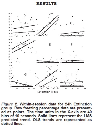
Figure 2 shows the raw data, OLS and robust LMS regression lines for each animal (A through I) in the 24 hr. Extinction group. As can be seen, LMS estimation results in steeper regression lines for most subjects, especially for those such as Subject G, with an unusually high freezing score towards the end of the extinction session. A similar, although less pronounced pattern may be observed for Subjects E and F. Estimation method aside, the analysis of the individual data clearly shows how repeated non-reinforced exposure to the CS resulted in sensitization, rather than extinction of the CS in six (A, B, C, D, H, I) out of nine subjects, which results in positive, rather than negative slopes.
For the 48 hour extinction group (Figure 3), this difference in the steepness of the OLS and LMS regression lines is even more pronounced, as can be seen in Subjects B, C, E, F, G, H and I. In each of these cases, unusually high freezing scores towards the end of the session flatten out the OLS regression lines, while the LMS remain unaffected: a sign of their robustness. In extreme cases, such as in subject D, this may even result in slopes of opposite signs for OLS and LMS estimations.
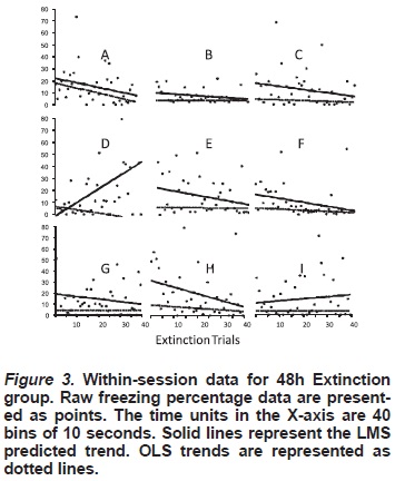
Summarizing the results from the first step of the analysis, LMS slopes show how extinction in the 24 hour group predominantly resulted in sensitization to the CS and only for the 48 hour group did it result in loss of conditioned responding for most subjects.
Comparison of OLS and LMS lines for within-session data.
Analyzing individual curves provides additional information about floor and ceiling effects on the within-session dynamics. Differences in conditioning levels (freezing response levels), limit or even condition the direction of the within-session trend. Too high initial values allow for sharper decline trends while low initial values favor flat or positive trends. This may be seen in the correlation between intercepts and slopes for LMS estimates. For the 24h group rab=-0.122, and for 48h rab=-0.858. The stronger correlation in the 48h group indicates that initial session values are more critical for this group. This analysis illustrates a common assumption of many computational models of Pavlovian conditioning, namely, the error correction nature of conditioning and extinction. This feature is best illustrated by the Rescorla-Wagner model (Rescorla & Wagner, 1972), where the magnitude of the associative change in each trial is proportional to the difference between the associative strength in the previous trial and the asymptotic value of conditioning or extinction in the present trial (l-SVit). Hence, for extinction trials (where l=0), the higher the previous level of conditioning (estimated here by the intercept of the regression line) the greater the loss in associative strength (the steeper the slope).
Conventional Analysis of Median Freezing Percentage (MFP)
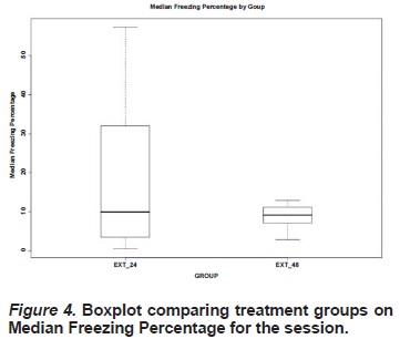
Average MFP was 20.01 (sd=19.7) for the 24h Extinction group and 8.65 (sd=3.4) for the 48h group. The Bartlett test for homogeneity of variances indicates the presence of heteroscedasticity, (K2 = 16.39, p< 0.001). This can be observed in the boxplots as well (Figure 4). Consequently, group comparison had to be corrected for lack of equivalence of the variances.
A variance-stabilization transformation (ln(x)) was used, and linear modeling (ANOVA) was applied to the transformed variable. This resulted in F(1,16)=1.59, p=0.225. Robust tests were performed, and both a permutation tests for means and a Wilcoxon/Mann-Whitney rank-sum tests yielded non-significant differences between groups. Mean difference derived from the asymptotic permutation test resulted in a standard z=1.62.
Group comparison using LMS slopes
The average LMSb for the 24h group was 0.448 (sd=0.723), and for the 48h group was -0.110 (sd=0.142). It is important to notice that many of LMSb values are negative (as expected in an extinction trend), which results in apparently large standard deviations as compared with the mean values. Consistent with the MFP results, the 24h group shows more dispersion than the 48h. Bartlett test for equality of the variances show significant differences in group variances (K2 = 14.608, p <0.001), requiring correction of lack of homoscedasticity.
The boxplot (Figure 5) shows the differences in dispersion for both groups. Additionally, compared with Figure 3, the difference between both extinction groups is sharper for LMSb.
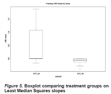
The ANOVA results on the log-transformed LMSb were F(1,16)=6.364, p=0.023. Significant results were obtained with both permutation test for means (z= 2.04) and Wilcoxon/Mann- Whitney rank-sum test (p<0.05).
ANOVA analyses were preferred over t-test, simply for practical reasons, to take advantage of standard linear modeling diagnosis procedures built-in on standard software routines. T-test performed on this data will yield exactly the same conclusions.
Comparison of MFP and LMSb results
Beyond the difference in statistical significance in favor of LMSb, the F value for LMSb was more than 4 times the F value for MFP, which for larger samples can translate into greater differences in statistical significance.
Regarding the clarity of the mean differences, in terms of interpretation, for MFP there’s a difference between 20 and 9 percentage freezing (in round numbers), which indicates the 48h extinction group shows a steeper extinction (response decrease). LMSb coeficients give results in the same direction but with different implications. According to the average slope for the 24h group, there’s no extinction on “average”, given that the trend is positive: Roughly speaking, there’s an increase of 1 freezing percentage point for each 2 bins, while the 48h group shows on average, a negative trend, which indicates a decrease of the fear response over time at an approximate rate of 1 percentage point each 10 bins.
LMSb results can give the appearance of being more difficult to interpret; however, they only show the need to visualize the individual extinction curves before interpreting the group analysis.
Regarding linear model diagnosis, both residual vectors were tested for normality (Royston, 1995), with non-significant departure from a normal distribution according to the W test, which is remarkable especially for a small sample. Checking for serial dependence on the residuals, Durbin-Watson tests for both models yielded non-significant results, indicating lack of serial dependence in model residuals. In summary, model residuals yielded similar results, indicating that neither option had a significant impact on the residuals compared with each other; both normality and serial independence of residuals check out well for both models.
DISCUSSION
There’s a sharp contrast in effect size between both procedures. Using LMSb as an outcome instead of MFP yielded much larger F-ratio. Both outcome variables in their original form are heteroscedastic across groups, requiring a variance-stabilizing transformation. This means there is no difference between both kinds of within-session summarization in terms of variance equivalence. However, differences in variances can be considered part of treatment effects. The homogenization of the 48h extinction group can be due to stronger effect of this treatment level. Using linear modeling assuming equal variances is a standard practice, and for this reason ANOVA results were presented, instead of using a more complex model assuming unequal variances.
Nevertheless, once the variances were stabilized via transformation, the results are very clear. Another aspect in which both outcomes resulted in very similar patterns is in residual diagnostic checks. Both residual analyses indicate there is not a major impact in choosing one outcome over another in terms of model diagnostics. This is important, because a more complicated quantity such as LMSb could be associated with issues with the distribution of the residuals, and in this case it proves to be similar to the use of a standard summary such as MFP.
The extreme difference in F-ratios indicates that using the LMS slopes captures differences between groups that escape MFP. Extinction curve linear slope measures a key feature of extinction dynamics over time: the steep decline of the fear response. Another factor contributing with the difference in F-ratios is the impact of the extreme variability in the 24h group on both models. The extreme difference in both Fvalues could be a result of the combination of the sensitivity of the slopes to treatment effects and a combination of the variance-stabilizing transformation with group differences. To avoid basing conclusions solely on this ANOVA results, permutation tests for means were carried out with the raw (non-transformed) outcome variables. For those results, LMSb effect size is 1.41 times larger instead of 4 times larger. Both results favor the LMS slope as an outcome variable that is more sensitive to treatment effects.
Beyond the differences in effect size in the between-group analysis, there’s something to be said about analyzing individual extinction curves and obtaining slopes for each subject. Analyzing within-subject performance has been a traditional staple of the experimental analysis of behavior (Sidman, 1960): molecular changes in the probability of responding were formerly privileged behavioral data under this conceptual framework, but were gradually displaced by more molar data and data representations (Skinner, 1976). It has long been known how averaging individual curves largely distorts the dynamics of performance; it is not uncommon to find that the average curve is very different from all the individual within-subject curves. In the present example, the average extinction curve for the 24hr group would have yielded little extinction, but would have obscured the fact that most subjects exhibited sensitization, rather than extinction to the repeated presentation of the CS.
The relationship between inter-individual variation and intra-individual variation has recently been revisited from an individual difference perspective. Molenaar (Molenaar, 2007; Molenaar, Sinclair, Rovine, Ram & Corneal, 2009), has argued that the former type of variability can only provide information on the latter under certain conditions, know as conditions of ergodicity. The conditions of ergodicity are twofold: on one hand the population of subjects has to be homogeneous, that is, all subjects have to conform to the same statistical model, and on the other the individual time series must be stationary (there must be an absence of trend trough time). Although arguments can be made in favor and against the compliance of the homogeneity condition for extinction data, the stationarity of the timeseries constitutes an insurmountable difficulty, since these data are expected to exhibit a decrease with time. Extinction data are clearly non-ergodic, and therefore demand an analytical approach which highlights individual variation but allows for group comparisons. The additional information yielded by this first analytical step provided insights that simply cannot be represented by a session total or average.
Regarding the advantages of using a robust regression procedure, the individual regression lines show the weakness of OLS for estimating trends for this data, and how using a robust procedure such as LMS can help to estimate a trend which captures the key feature of the within-session data.
FINAL COMMENTS
The results demonstrate several advantages of the application of the LMS robust regression technique within a 2-step procedure to fear conditioning extinction data, as compared with standard one-way mean-difference analyses of session totals. It is important to highlight this procedure is just a good option to overcome the limitations of simple linear modeling of session totals. Many of the problems are mitigated or dealt with in a coherent way. However, this is not equivalent to saying this is a final or automatic solution. Individual dynamics cannot be reduced to a simple linear slope. A processmodel of extinction may be needed in some cases, and its incorporation into a statistical analysis may require more complex and flexible modeling techniques.
Following the state of the art, with journals publishing standard statistical results for extinction experiments, even a slight improvement in the analysis can be of great benefit. In this sense, robust regression integrated into the 2-step analysis shows to have several advantages, including larger effect size, arguably due to an improved signal-to-noise ratio and more meaningful results in terms of extinction process and the visualization of individual withinsession extinction data. Those improvements are evident even in worst-case scenario type of data from a real experiment, in the presence of outliers and with a small sample size.
Further studies are required to explore the application of robust regression or specifically LMS to extinction data, such as extensive simulation studies and more examples with real data. This study shows, within the limitations of a single dataset, the benefits of improving standard analysis with robust slopes for the analysis of fear response extinction data.
REFERENCES
1. Adichie, J. N. Use of ranks for testing coincidence of several regression lines. Annals of Statistics, 3(2), (1975), 521-527. [ Links ]
2. Brooks, D. C., Vaughn, J. M., Freeman, A. J. & Woods, A. M. An extinction cue reduces spontaneous recovery of ataxic ethanol tolerance in rats. Psychopharmacology, 176(3-4), (2004), 256-265. [ Links ]
3. de Leew, J. & Meijer, E. Handbook of multilevel analysis. New York: Springer, (2008). [ Links ]
4. Deleeuw, J. & Kreft, I. G. G. Questioning multilevel models. Journal of Educational and Behavioral Statistics, 20(2), (1995), 171- 189. [ Links ]
5. Hampel, F. R. General qualitative definition of robustness. Annals of Mathematical Statistics, 42(6), (1971), 1887-&. [ Links ]
6. Hubert, M., Rousseeuw, P. J. & Van Aelst, S. High-breakdown robust multivariate methods. Statistical Science, 23(1), (2008), 92-119. [ Links ]
7. James, G. M. & Sood, A. Performing hypothesis tests on the shape of functional data. Computational Statistics & Data Analysis, 50(7), (2006), 1774-1792 [ Links ]
8. Killeen, P. R., Sanabria, F. & Dolgov, I. The Dynamics of Conditioning and Extinction. Journal of Experimental Psychology- Animal Behavior Processes, 35(4), (2009), 447-472. [ Links ]
9. Ledgerwood, L., Richardson, R. & Cranney, J. D-cycloserine and the facilitation of extinction of conditioned fear: Consequences for reinstatement. Behavioral Neuroscience, 118(3), (2004), 505-513. [ Links ]
10. Li, T. & Balakrishnan, N. Best linear unbiased estimators of parameters of a simple linear regression model based on ordered ranked set samples. Journal of Statistical Computation and Simulation, 78(12), (2008), 1265-1276. [ Links ]
11. Ludbrook, J. Linear regression analysis for comparing two measurers or methods of measurement: But which regression? Clinical and Experimental Pharmacology and Physiology, 37(7), (2010), 692-699. [ Links ]
12. Mackintosh, N. J. Theory of attention - variations in associability of stimuli with reinforcement. Psychological Review, 82(4), (1975), 276-298. [ Links ]
13. McAleer, M., Chan, F., Hoti, S. & Lieberman, O. Generalized Autoregressive Conditional Correlation. Econometric Theory, 24(6), (2008), 1554-1583. [ Links ]
14. Molenaar, P. Psychological methodology will change profoundly due to the necessity to focus on intra-individual variation. Integr Psychol Behav Sci, 41(1), (2007), 35-40; 75-82. [ Links ]
15. Molenaar, P., Sinclair, K., Rovine, M., Ram, N. & Corneal, S. Analyzing developmental processes on an individual level using nonstationary time series modeling. Dev Psychol, 45(1), (2009), 260- 271. [ Links ]
16. Mount, D. M., Netanyahu, N. S., Romanik, K., Silverman, R. & Wu, A. Y. A practical approximation algorithm for the LMS line estimator. Computational Statistics & Data Analysis, 51(5), (2007), 2461-2486. [ Links ]
17. Myers, K. M. & Davis, M. Mechanisms of fear extinction. Molecular Psychiatry, 12(2), (2007), 120-150. [ Links ]
18. Ozdemir, Y. A. & Esin, A. A. Best linear unbiased estimators for the multiple linear regression model using ranked set sampling with a concomitant variable. Hacettepe Journal of Mathematics and Statistics, 36(1), (2007), 65-73. [ Links ]
19. Pearce, J. M. & Hall, G. A Model For Pavlovian Learning - Variations In The Effectiveness Of Conditioned But Not Of Unconditioned Stimuli. Psychological Review, 87(6), (1980), 532-552. [ Links ]
20. Rescorla, R. A. Pavlovian conditioning and its proper control procedures. Psychological Review, 74(1), (1967), 71-&. [ Links ]
21. Rescorla, R. A. Summation: Assessment of a configural theory. Animal Learning & Behavior, 25(2), (1997), 200-209. [ Links ]
22. Rescorla, R. A. Are associative changes in acquisition and extinction negatively accelerated? Journal of Experimental Psychology- Animal Behavior Processes, 27(4), (2001), 307-315. [ Links ]
23. Rescorla, R. A. Spontaneous recovery from over expectation. Learning & Behavior, 34(1), (2006), 13-20. [ Links ]
24. Rescorla, R. A. & Wagner, A. R. A theory of Pavlovian conditioning: Variations in the effectiveness of reinforcement and non reinforcement. In A. H. B. a. W. F. Prokasy (Ed.), Classical Conditioning II: (1972), (pp. 64-99). New York: Appleton Century Crofts. [ Links ]
25. Richardson, R., Ledgerwood, L. & Cranney, J. Facilitation of fear extinction by D-cycloserine: Theoretical and clinical implications. Learning & Memory, 11(5), (2004), 510-516. [ Links ]
26. Rousseeuw, P. J. Least Median of Squares Regression. Journal of the American Statistical Association, 79(388), (1984), 871-880. [ Links ]
27. Royston, P. A remark on algorithm as-181 - the w-test for normality. Applied Statistics-Journal of the Royal Statistical Society Series C, 44(4), (1995), 547-551. [ Links ]
28. Sen, P. K. Class of aligned rank order tests for identity of intercepts of several regression lines. Annals of Mathematical Statistics, 43(6), (1972), 2004-2012. [ Links ]
29. Sidman, M. Tactics of scientific research; evaluating experimental data in psychology. New York,: Basic Books, (1960). [ Links ]
30. Skinner, B. F. Farewell, My Lovely. Journal of the Experimental Analysis of Behavior, 25(2), (1976), 218-218. [ Links ]
31. Tabatabai, M. A. & Tan, W. Y. Some comparative-studies on testing parallelism of several straight-lines under heteroscedastic variances. Communications in Statistics-Simulation and Computation, 14(4), (1985), 837-844. [ Links ]
32. Tate, R. Interpreting hierarchical linear and hierarchical generalized linear models with slopes as outcomes. Journal of Experimental Education, 73(1), (2004), 71-95. [ Links ]
33. Tian, Y. G. & Wiens, D. P. On equality and proportionality of ordinary least squares, weighted least squares and best linear unbiased estimators in the general linear model. Statistics & Probability Letters, 76(12), (2006), 1265-1272. [ Links ]
34. Vargas-Irwin, C. & Robles, J. R. Effect of sampling frequency on automatically-generated activity and freezing scores in a Pavlovian fear-conditioning preparation. Revista Latinoamericana de Psicología, 41(2), (2009), 187-195. [ Links ]

