Introduction

In the last decades, important advances have been made in the study of the gravitomagnetic clock effect. Beginning with the seminal work by Cohen and Mashhoon ^[1]. In which they presented the influence of the gravitomagnetic field to the proper time of an arbitrary clock about a rotating massive body. In their paper, Cohen and Mashhoon, also showed the possibility of measuring this effect. In this work, we present a theoretical value for the gravitomagnetic clock effect of a spinning test particle orbiting around a rotating massive body.

According with the literature, we find different complementary ways that study the phenomena in regard to the gravitomagnetism clock effect. The first way take two family of observers. The first is the family of static observer (or threading observers) with four-velocity m = M ^-1 d _t and world lines along the time coordinate lines. The second famili is the ZAMO's (or slicing observers) with four-velocity n = N ^-1 {∂ _t - Ν ^φ ∂ _φ ) and world lines orthogonal to the time coordinate hypersurfaces ^[2-4]. They obtain, in the threading point of view, the local spatial angular direction as

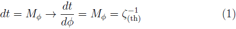
which gives an inverse angular velocity or the change with respect to angle of the time coordinate. Since is angular velocity, Bini et al. integrate the coordinate time for one complete revolution both in a direction and in opposite direction ^[2]. Then the physical components of the velocities are related to the coordinate angular velocity.

This group study the case when the particle has spin. They take the Frenet-Serret frame (FS) associated to worldline of the test particle and calculates with help of the angular velocity the evolution equation of the spin tensor in terms of the FS intrinsic frame ^[5,6]. The work of this group considers the MPD equations and their su-pplementary conditions for the spin and give their answer in terms of angular velocity.

The second group integrates around a closed contour. They take the time for this loop when the test particle rotates in clockwise and the test particle in opposite sense ^[1,7].

A third group deduces the radial geodesic equation from the line element in the exterior field of a rotating black hole. With this equation yields the solution and calculate the inverse of the azimuthal component of four velocity. Then they introduce the first order correction to the angular velocity

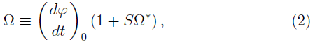
and obtain the differentiate between prograde and retrograde orbits and integrate from zero to 2π. The clock effect is the difference of theses two orbits ^[8-10].

The fourth group takes some elements of electromagnetism and does an analogy between Maxwell equations and Einstein linealized equations ^[11-19]. Finally the group that makes a geometric treatment of the gravitomagnetic clock Effect ^[20,21].

According with other papers that work the MPD equations, the novelty of our work is that we calculate numerically the full set of MPD equations for the case of a spinning test particle in a Kerr metric. Secondly, we take the spin without restrictions in its velocity and spin orientation. In the paper by Kyrian and Semerak the third example is refered to the particular case when the spin is orthogonal to the equatorial plane in a Kerr metric ^[22].

In this paper, our aim, it is not only describing the trajectories of spinning test particles, but also to study the clock effect. Therefore, we calculate numerically the trajectory both in a sense and in the other for a circular orbit. We measure the delay time for three situations: two spinless test particles are traveling in the same circular orbit, two spinning test particles with its spin value orthogonal to equatorial plane and two spinning test particles without restrictions in its spin orientation.

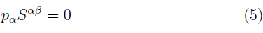
In this paper, we use the set of Mathisson-Papapetrou-Dixon equations presented by Plyatsko, R. et al. ^[23] and extend this approach, considering the spin of the particle without restrictions in its orientation, while Plyatsko et al. only take a constant value for the spin in its magnitude and orientation; we allow both to be varied, using the full set of MPD equations and the Mathisson-Pirani (MP) supplementary spin condition. In the literature, one can find different conditions to fix the center of mass, leading to different kinematical behaviours of the test particles. One of the features of the MPD equations is the freedom to define the representating worldline to which u ^α is tangente vector. Therefore the worldline can be determined from physical conside-rations. The first condition is the Mathisson-Pirani condition (MP, 1937):

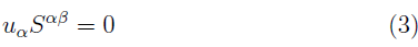
in this condition the reference worldline is the center of mass as measured in the rest frame of the observer of velocity u ^{α [24,25]}. This condition does not fix a unique worldline and u ^α is uniquely defined by ρ ^α and S ^αβ . If one uses this condition, the trajectory of the spinning test particle is represented by helical motions. Costa et al. ^[26] explain that these motions are physically possible. We use this condition when working with the MPD equations in the case of a spinning test particle orbiting a rotating massive body. The second condition is presented by Corinaldesi and Papapetrou (CP, 1951) which is given by

which depends on coordinates. For this condition, the worldline is straight and its tangent u ^α is parallel to the four momentum ρ ^{μ [22]}.

The third condition is introduced by Tulczyjew and Dixon (TD, 1959) and written which is given by

where

is the four momentum. This condition implies that the worldline is straight and its tangent u ^α is parallel to ρ ^α and the spin is constant ^[27]. This condition is cova-riant and guarantees the existence and uniqueness of the respective worldline ^[28].

The fourth is given by Newton and Wigner (NW) which is a combination of the TD and MP conditions

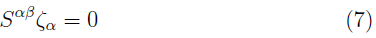
with ζ _α : = ρ _α + Muα and uα being a timelike vector. This condition provides an implicit relation between the four-momentum and the wordline's tangent vector.

The fifth condition is called Ohashi-Kyrian-Semerak (OKS, 2003):

where w ^α is some time-like four vector which parallely transports along the representative worldline ^[22]:

For the study of spinning test particles, we use the equations of motion for a spinning test particle in a gravitational field without any restrictions to its velocity and spin orientation ^[23]. In this paper, we use the MPD equations presented by Plyatsko, R. et al. ^[23]. They yield the full set of Mathisson-Papapetrou-Dixon equations (MPD equations) for spinning test particles in the Kerr gravitational field ^[23], where they integrate nume-rically the MPD equations for the particular case of the Schwarzschild metric.

For the scope of this work, we will take the MPD equations of motion for a Kerr metric, and additionally we will include the spin of the test particle. This calculation has been made with the Mathisson-Pirani supplementary condition; the trajectories have been obtained by numerical integration, using the Runge-Kutta algorithm ^[29].

Presently, there exists an interest in the study of the effects of the spin on the trajectory of test particles in rotating gravitational fields ^[30]. The importance of this topic increases when dealing with phenomena of astrophysics such as accretion discs in rotating black holes, gravitomagnetics effects ^[8] or gravitational waves induced by spinning particles orbiting a rotating black hole ^[31,32]. The new features of the spin-gravity coupling for highly relativistic fermions are considered in ^[33] and ^[34].

The motion of particles in a gravitational field is given by the geodesic equation. The solution to this equation depends on the particular conditions of the problem, such as the rotation and spin of the test particle, among o-thers; therefore there are different methods for its solution ^[35,36].

Basically, we take two cases in motion of test particles in a gravitational field of a rotating massive body. The first case describes the trajectory of a spinless test particle, and the second one the trajectory of a spinning test particle in a massive rotating body. In the case of the spinless test particles, some authors yield the set of equations of motion for test particles orbiting around a rotating massive body. The equations of motion are considered both in the equatorial plane ^[37-39], and in the non-equatorial plane ^[38,40,41] (Kheng, L., Perng, S., and Sze Jackson, T.: Massive Particle Orbits Around Kerr Black Holes. Unpublished). For the study of test particles in a rotating field, some authors have solved for particular cases the equations of motion both for spinless and for spinning test particles of circular orbits in the equatorial plane of a Kerr metric ^{[20,31,37,42-46]}.

With the aim of proving the equations of motion with which we worked, solve numerically the set of equations of motion obtained via MPD equations both for the spinless particles and for spinning particles in the equatorial plane and will compare our results with works that involve astronomy, especially the study of spinning test particles around a rotating central source. We take the same initial conditions in the two cases for describing the trajectory of both a spinless particle and a spinning particle in the field of a rotating massive body. Then, we compare the Cartesian coordinates (x, y, z) for the trajectory of two particles that travel in the same orbit but in opposite directions.

For the numerical solution, we give the full set of MPD equations explicitly, while that Kyrian and Semerak only name them. Also, we give the complete numerical solution. Kyrian and Semerak integrate with a step of M/100 = 1 χ 10^-2 while we integrate with a step of n = 2^-22 = 2.384 1 85 χ 10^-7. In the majority of cases, the solutions are partial because it is impossible to solve analytically a set of eleven coupled differential equations. The recurrent case that they solve is a spinning test particle in the equatorial plane and its spin value is constant in the time (S_┴ =constant).

This work is organized as follows. In Section 2 we give a brief introduction to the MPD equations that work the set of equations of motion for test particles, both spinless and spinning in a rotating gravitational field. From the MPD equations, we yield the equations of motion for spinless and spinning test particles. Also, we will give the set of the MPD equations given by Plyatsko et al. ^[23] in schematic form to work the equations of motion in a Kerr metric. In Section 3 and 4, we present the gravitomagnetic clock effect via the MPD equations for spinless and spinning test particles. Then, in Section 5, we perform integration and the respective numerical comparison of the coordinate time (t) for spinless and spinning test particles in the equatorial plane. Finally we make a numerical comparison of the trajectory in Cartesian coordinates for two particles that travel in the same orbit, but in opposite directions. In the last section, conclusions and some future works. We shall use geometrized units; Greek indices run from 1 to 4 and Latin indices run from 1 to 3. The metric signature (-,-,-,+) is chosen.

Introduction to the Mathisson-Papapetrou-Dixon equations

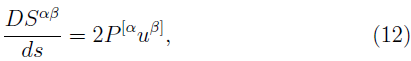
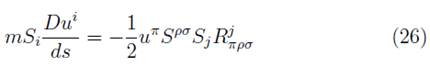
In general the MPD equations ^{[24,27,47,48]} describe the dynamics of extended bodies in the general theory of relativity which includes any gravitational background. These equations of motion for a spinning test particle are obtained in terms of an expansion that depends on the derivatives of the metric and the multipole moments of the energy-momentum tensor (T ^μν ) ^[27] which describes the motion of an extended body. In this work, we will take a body small enough to be able to neglect higher multipoles. According to this restriction the MPD equations are given by

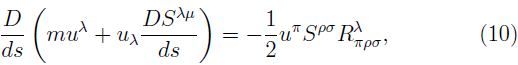
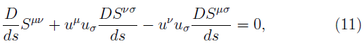
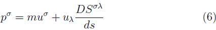
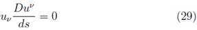
where the covariant derivative is given by D/ds, the antisymmetric tensor , S ^µv , R ^λ _ϖpσ is the curvature tensor, and υ ^μ = dz ^μ /ds is the particle's four-velocity. We do not have the evolution equation for υ ^μ and it is necessary to single out the center of mass which determines the world line as a representing path and specifies a point about which the momentum and spin of the particle are calculated. The worldline can be determined from physical considerations ^[49]. In general, two conditions are typically imposed: The Mathisson-Pirani supplementary condition (MP) u _σ S ^µσ = 0 ^[24,25] and the Tulczyjew-Dixon condition ρ _σ = 0 ^[27]. We found that if we contract the equation

with the four velocity u ^α , we obtain

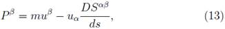
where m = -P ^α u _α . Given the MP condition, the four momentum is not para-llel to its four velocity u ^β ; therefore, it is said to possess "hidden momentum". This last equation can be written as

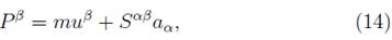
where a ^α = Du ^α /ds is the acceleration. This acceleration results from an interchange between the momentum mu ^β and hidden momentum S ^αβ a _α . These variations cancel out at every instant, keeping the total momentum constant ^[75]. The above equation can be expressed as

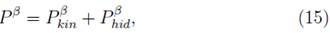
where P ^β _kin = mu ^β is the kinetic momentum associated with the motion of the centroid and the component P ^β _hid = S ^αβ a _α is the hidden momentum. In this case, if the observer were in the center of mass, he would see its centroid at rest then we would have a helical solution.

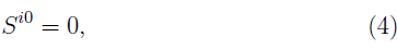
To obtain the set of MPD equations, we take the MP condition which has three independent relationships between S ^μσ and u _σ . By this condition S ⁱ⁴ is given by

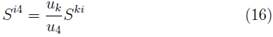
with this expression we can use the independent components S ^ik . Sometimes for the representation of the spin value, it is more convenient to use the vector spin, which in our case is given by

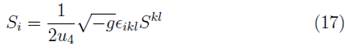
where Є _ikl is the spatial Lèvi-Cività symbol.

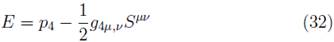
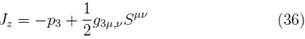
When the space-time admits a Killing vector ξ ^υ , there exists a property that includes the covariant derivative and the spin tensor, which gives a constant and is given by ^[50]

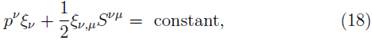
where p ^v is the linear momentum, ξ _ν,μ is the covariant derivative of the Killing vector, and S ^vµ is the spin tensor of the particle.

In the case of the Kerr metric, one has two Killing vectors, owing to its stationary and axisymmetric nature. In consequence, Eq. (18) yields two constants of motion: the total energy E and the component z of the angular momentum J ^[51].

MPD equations for a spinning test particle in a metric of a rotating body

Given that the spinning test body is small enough compare with the characteristic length, this body can be considered as a test particle. In this section, the equations of motion (Eqs. 10 and 11) of the test particle are firstly introduced in the case when the particle is orbiting in an axisymmetric and stationary spacetime. Then, we specify the equations of motion for the case of a spinning test particle for a Kerr metric.

According to R.M. Plyatsko et al. ^[23], the full set of the exact MPD equations of motion for a spinning test particle in the Kerr field, if the MP condition (3) is taken into account, obtain a general scheme for the set of equations of motion for a spinning test particle in a rotating field. Plyatsko et al. ^[23] use a set of dimensionless quantities y to achive this. In particular, the Boyer-Lindquist coordinates are represented by

the corresponding four-velocity are given by

and the spatial spin components by ^[52]

where M is the mass parameter of the Kerr spacetime. m is the mass of a spinning particle, a constant of motion for the MP SSC and implies that

In addition, they introduce the dimensionless quantities

representing the proper time s and the constants of motion: Energy (E) and the angular momentum in the z direction (J _z ).

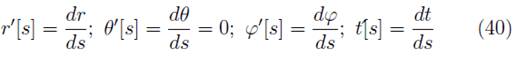
The set of the MPD equations for a spinning particle in the Kerr field is given by eleven equations. The first four equations are

where the dot denotes the usual derivative with respect to x.

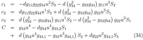
The fifth equation is given by contracting the spatial part of equation (10) with S_i (λ = 1, 2, 3). The result is multiplied by S ₁ S ₂ , S ₃ and with the MP condition (3) we have the relationships ^[53]:

then we obtain

which can be written as

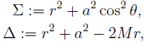
where

where g is the determinant of the metric g _µv .

The sixth equation is given by

which can be written as

where

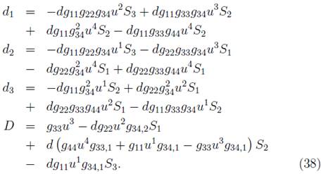
The seventh equation is given by

which can be written as

where

with

where g is the determinant of the metric g _µv and the values of g ₁₁,g ₂₂,g ₃₃, ··· are the components of the metric g _µv .

The eighth equation is given by

which can be written as

where

Finally, the last three equations are given by

which give the derivatives of the three spatial components of the spin vector (Ṡ _i ): ẏ₉, ẏ₁₀ ẏ₁₁ and The full set of the exact MPD equations for the case of a spinning test particle in a Kerr metric under the Pirani condition (3) is in the appendix of ^[23].

After achieving a system of equations of motion for spinning test particles, we solve them numerically. We use the fourth-order Runge Kutta method for obtaining the Cartesian coordinates of the trajectories (x, y, z). For our numerical calculations, we take the parameters both of the central mass and the test particle such as the radio, the energy, the angular momentum and the components of the four velocity (u ^µ ). We calculate the full orbit in Cartesian coordinates (x, y, z) of a test particle around a rotating massive body for both spinless and spinning test particles. Then, we make a comparison of the time that a test particle takes to do a lap in the two cases.

Equations of motion for a spinning test particle orbiting a massive rotating body

In the last section, we obtained the general scheme for the set of equations of motion of a spinning test particle in the gravitational field of a rotating body ^[54]. Now, we consider the case for the equatorial plane, which is given by the following set of equations:

where; is the proper time.

For our numerical calculation, we separate from the full set of equations each one of the functions for the four velocity vector (dx ^µ /ds) and the differentials for the spatial components of spin vector (S _i ). Finally from the eleven differential equations, we obtain the trajectories of the spinning test particle orbiting around the rotating central mass (M). We perform our numerical integration as follow: In the first one, we perform the integration along the direction of the rotation axis of the massive body, and the second one in its opposite sense. The value of the components from initial four velocity vector is obtained by replacing the values of the constants of motion (E and J), the Carter's constant (Q) and the radio in the Carter's equations ^[35]

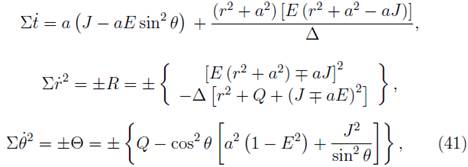
where J, E and Q are constants and

M and α = J/M are the mass and specific angular momentum for the mass unit of the central source.

The Carter's constant (Q) is a conserved quantity of the particle in free fall around a rotating massive body. This quantity affects the latitudinal motion of the particle and is related to the angular momentum in the O direction. From (41), one analyzes that in the equatorial plane, the relation between Q and the motion in O is given by

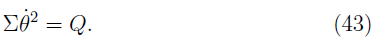
When Q = 0 corresponds to equatorial orbits and for the case when Q ≠ 0, one has non-equatorial orbits.

MPD equations for a spinless test particle in a Kerr metric

The traditional form of MP equations is given by the Eq (10)^[24] and for our problem, we consider the motion of a spinning test particle in equatorial circular orbits (θ = π/2) of the rotating source. For this case, we take ^[55]

when the spin is perpendicular to this plane and the MP condition (3), with

The equation is given by

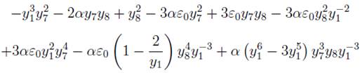
where y₁ = r/M, y₇ = Mu ³, y₈ = u⁴, ε₀ = |S₀| /mr and α = α/M. When the particle does not have spin (ε₀ = 0), the set of equations (10) with the dimensionless quantities y _i (19) and (20) is given by

In addition to Eq. (47), we take the condition u _µ u ^µ = 1 and obtain

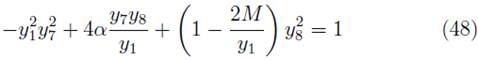
We solve the system of equations (47) and (48) for the case of a circular orbit and obtain the values of y₇ = Mu ³ and y ₈ = u ⁴ in the equatorial plane.

Gravitomagnetic effects for spinning test particles

In the study of the gravitomagnetic effects, we find the gravitomagnetic force is the gravitational counterpart to the Lorentz force in electromagnetics. Hence, there is an analogy between classical electromagnetism and general relativity such as the possibility that the motion of mass could generate the analogous of a magnetic field. ^[56]. In general relativity, the gravitomagnetic field is caused by mass current and has interesting physical properties which explain phenomena such as the precession of gyroscopes or the delay time for test particles in rotating fields ^[57].

In this section, we describe some phenomena of the trajectories from the spin vector, represented by a gyroscope, with the help of the gravitomagnetic effects such as the clock effect, Thomas precession, Lense-Thirring effect or Sagnac effect ^[43,58,59].

The first effect that we take is the Lense - Thirring effect which has the consequence that moving matter should somehow drag with itself nearby bodies. We can do an analogy of this dragging of mass current with a magnetic field produced by a charge in motion. With this analogy, we set up two spinning test particles orbiting in an equatorial plane of a rotating gravitational field. Then, we compare the trajectories of these two spinning test particles that travel in opposite directions in the same circular orbit. We found that one of the particles arrived before the other one. The delay time is due not only to the dragging of the frame system, but also to the angular motion of the spinning test particle ^[8]. On the other hand, the rotating massive body induces rotation and causes the precession of the axis of a gyroscope which creates a gravitomagnetic field.

The form of the figure is the same, either that the spinning particle orbits in the direction of the central mass or in opposite direction, but they are out of phase in the space.

Gravitomagnetic clock effect for spinning test particles

In the scond half of the nineteenth century, Holzrrrüller ^[60] and Tisserand ^[61] with the help of works in electrodynamics, postuled a gravitomagnetic component for the gravitational influence of the Sun on the motion of planets. The general relativistic effect of the rotation of the Sun with regard to the planetary orbits was calculated by de Sitter ^[62] and later by Lense and Thirring ^[63]. After, Ciufolini described the Lense-Thirring precession of satellites such as LAGEOS and LAGEOS II around the rotating Earth ^[64]. Then NASA launched a satellite around of the Earth. This satellite was orbiting in the polar plane and carried four gyroscopes whose aim was to measure the drag of inertial systems produced by mass current when the Earth is rotating and to measure the geodesic effect given by curvature of the gravitational field around the Earth ^[65]. This experiment was called Gravity Probe B.

There is a phenomenon called the gravitomagnetic clock effect which consists in a difference in the time which is taken by two test particles to travel around a rotating massive body in opposite directions in the equatorial plane ^[8]. This effect involves the difference in periods of two test particles moving in opposite directions on the same orbit. Let τ₊ (τ ^_) be the proper period that it takes for a test particle to complete a lap around a rotating mass on a prograde (retrograde) orbit. In the literature, the majority of works that study the clock effect consider the difference of periods for spinless test particles. In this paper, we study the clock effect for two spinning test particles orbiting around to a rotating body in the equatorial plane.

To check our results, we review the papers regarding gravitomagnetic clock effect ^[66] and compare their results with ours. The delay time given by the clock effect is t ₊ - t_ = 4ϖα/c, where α = J/Mc is the angular momentum density of the central mass. Tartaglia has studied the geometrical aspects of this phenomenon ^[20,67], and Faruque yields the equation of the gravitomagnetic clock effect with spinning test particles as ^[8]

where S₀ is the magnitude of the spin.

In true units this relation is given by

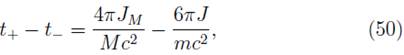
where the first relation of the right could be used to measure J/M directly for an astronomical body; in the case of the Earth t₊ - t _ 10^-7s, while for the Sun t₊ - t_ 10^-5s ^[18].

Numerical comparison for spinless and spinning test particle via MPD equations

We take the set of MPD equations for a spinning test particle in a Kerr me-tric given in the second section. This set is composed of eleven coupled di-fferential equations. We input the initial conditions in geometrized units as: E = 0.951906, r =10, α = 1, M =1, Carter's constant: Q = 0.000008 and angular momentum: J = 3.426929. With these initial values, we obtain the four-vector velocity (aV/ds) with the Carter's equations (⁴¹ - ⁴²). The spatial components of vector spin are used to obtain the integration limits. For our case, the spin components are: Si = 10_¹², S₂ = 0.1, S₃ = 0.1. Then, we integrate the set of eleven equations, which were presented in the section 2.1, with the fourth-order Runge-Kutta method ^[29] with a step size of 2.384185 χ 10^-7, while Kyrian and Semerák integrate with a step of M/100 = 1 χ 10^{-2 [22]}. With this code, we get the Cartesian coordinates for a circular orbit when the spinning test particle travels in the same direction of rotation of the central source (α) and when it orbits in opposite sense. We register the coordinate time (t = x⁴) that the test particle takes to do a lap in each sense of rotation. Finally, we take the delay time in these two laps and obtained in non-geometrized units

Our numerical result is in according with previous works ^[8,43,68], made of an analytic via. In this result, we found that the clock effect is reduced by the presence of the spin in the test particle. Both Mashhoon ^[43] and Faruque ^[9] develop an approximation method for studying the influence of spin on the motion of spinning test particles ^[69], while we use an integration method of the full set of MPD equations in order to obtain the value of the coordinate time (t).

This delay time is due to the drag of the inertial frames with respect to infinity and is called the Lense-Thirring effect ^[70]. In the case of the spinning test particles, there is not only a difference in the time given by the Lense-Thirring effect, but also by a coupling between the angular momentum of the central body with the spin of the particle ^[71]. The features change if the test particle rotates in one direction or the other; therefore, the period is different for one direction and for the other, and for whether or not the particle has spin.

Results of the spin vector

In regard to the spin tensor (S ^µV ), sometimes, for the numerical calculation, it is more convenient the spin vector (S _i ) which is given by the relationship (25). For our numerical calculations, we take the case when the spin is orthogonal to the equatorial plane, that is, S ₁ = 0, S ₂ ≠ 0 and S ₃ = 0. In this case, we present our main results with two graphs. For the case (S ₂ ≠ 0), the spin has a tiny nutation (Figure 1). The first graph shows the motion of the spin vector in Boyer-Lindquist coordinates (S ₁,S ₂,S ₃). Since both the radius (S ₁ ) and the azimuth angle are constant the spin vector describes an oscillating movement with a maximum height of 2 x10^-14. This oscillation is very short compared with the radius (r = 10) of the circle that describes the trajectory.

FIGURE 1: The bobbing of the spinning test particle with the Pirani condition (geometrized units) 

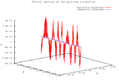
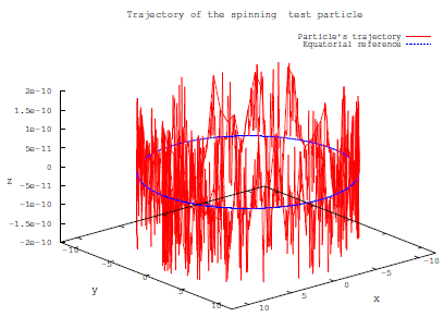
If we draw at the same time the orbital motion and the spin motion, we obtain an ascending and descending movement within an enveloping sinusoidal wave (Figure 2). This movement is called "bobbing" ^[73]. Moreover, this ascendant and descendent movement is due to the supplementary spin condition that we take to be the MP condition (S ^µV u _v = 0), where u _v is the center of mass four velocity. In this situation, the center of mass is measured in its proper frame (that is, the frame is at rest). This phenomenon is due to the shifting of the center of mass, and in addition, the momentum of the particle not being parallel to its four-velocity in general. There is a "hidden momentum" that produces this nutation. In an analogy with the electric (E) and magnetic (B) fields, there would be a E x B drift, that is, the motion is des-cribed by helical motions ^[74]. Costa et al. describe this physical situation due to the MP supplementary condition ^[75]. In the case that we are studying, the world tube is formed by all possible centroids which are determined by the MP spin supplementary condition. The size of this tube is the minimum size of a classical spinning particle without violating the laws of Special Relativity. Additionally, this world tube contains all the helical solutions within a radius R = S/M. The electromagnetic analogue of the hidden momentum is x which describes the bobbing of a magnetic dipole orbiting a cylindrical charge. Let the line charge be along the z axis, thethe electric field it and a charged test particle with magnetic dipole moment orbiting it. The particle will have a hidden momentum hid= χ and oscillates between positive and negative values along the z axis with ascendant and descendent movements in order to keep the total momentum constant. According with other papers that use the MPD equations, the novelty of our work is that we calculate numerically the full set of MPD equations for the case of a spinning test particle in a Kerr metric. Secondly, we take the spin without restrictions in its velocity and spin orientation. In the paper by Kyrian and Semerák the third example that they work, refers to the particular case when the spin is orthogonal to the equatorial plane in a Kerr metric ^[22]. On the other hand, our interest it is not only in to describe the trajectories of spinning test particles, but also to study the gravitomagnetic clock effect via the MPD equations. Therefore, we calculate numerically both trajectories, i.e., in the same and in the opposite way, in the case of a circular orbit. We measure the delay time for three different situations, namely, for the spinless test particle, traveling one way and the opposite, and for the spinning test particle for two different spin configuration. Regarding the spin configuration for the first, the spin has its value orthogonal to the equatorial plane of the trajectory, and for the second, the spin has no restrictions. For the numerical solution, we give the full set of MPD equations explicitly, while that Kyrian and Semerak only name them. Also, we give the complete numerical solution. In the majority of cases, the solutions are partial because it is impossible to solve analytically a set of eleven coupled differential equations. The recurrent case that they solve is a spinning test particle in the equatorial plane and its spin value is constant in the time (S _┴ = constant) ^[43].

FIGURE 2: The spinning test particle with the Pirani condition has a helical trajectory (geometrized units) 

Conclusions

In this paper, we take the Mathisson-Papapetrou-Dixon (MPD) equations yielded by Plyatsko et al. and apply them to the case of a spinning test particle orbiting around a rotating massive body in an equatorial plane. In addition, we yield a scheme for the eleven equations of the full set of equations of motion when the particle is orbiting any gravitational field. In the second part, we calculate the numerical solution of the trajectories in Cartesian coordinates (x, y, z) of the spinning test particles orbiting in a Kerr metric and compare the time of two circular orbits in the equatorial plane for two test particles that travel in the same orbit but in opposite directions. There is a delay time for a fixed observer relative to the distant stars. This phenomenon is called clock effect. For the case of the spinning test particles, this delay time is given not only by the angular momentum from the central mass, but also by the couple between the angular momentum from the massive rotating body and the parallel component of the spin of the test particle. In the MPD equations, this couple is given by the contraction between the components of the Riemman tensor (R ^µ _νρσ) and the spin tensor (S^ρσ ).

On the other hand, we obtained the graphs that describe both the orbital motion and the motion of the spin vector freely rotating in the polar component (S₂ ≠ 0). With this kind of motion, we make an analogy with the bobbing of a magnetic dipole in a electromagnetic field.

In the future, we will work on the set of equations of motion of a test particle both spinless and spinning for spherical orbits, that is, with constant radius and in non-equatorial planes in a Kerr metric. In addition, we are interested in relating these equations with the Michelson - Morley type experiments.