Services on Demand
Journal
Article
Indicators
-
 Cited by SciELO
 -
 Access statistics
Related links
-
 Cited by Google
 -
 Similars in
SciELO
 -
 Similars in Google
Share
Cuadernos de Economía
Print version ISSN 0121-4772
Cuad. Econ. vol.35 no.spe67 Bogotá Jan. 2016
https://doi.org/10.15446/cuad.econ.v35n67.52743
Sub-national fiscal policy under cooperative and non-cooperative models
Política fiscal subnacional con modelos cooperativos y no cooperativos
Politique fiscale infranationale avec des modèles coopératifs et non coopératifs
Política fiscal subnacional com modelos cooperativos e não cooperativos
Ligia Alba Melo-Becerraa
a The author is Senior Researcher of the Research Unit at Banco de la República (Central Bank of Colombia). She would like to express her gratitude to Michele Santoni for his helpful suggestions and comments. She also wishes to thank Helena González for her research assistance. The opinions expressed herein are those of the author, and do not necessarily reflect the views of Banco de la República or its Board of Directors. Correspondence: lmelobec@banrep.gov.co Banco de la República, Bogotá, Colombia.
Sugerencia de citación: Melo-Becerra, L. A. (2016). Sub-national fiscal policy under cooperative and non-cooperative models. Cuadernos de Economía. 35(67), 253-279. doi: 10.15446/cuad.econ.v35n67.52743.
Abstract
This article presents a comparative analysis of the optimal fiscal response to shocks in the sub-national public sector in cooperative and non-cooperative models. The analysis is undertaken by comparing models that assume idiosyncratic demandside shocks and sub-national autonomy to collect taxes, with models that assume that the central government collects the taxes of the whole country and redistributes them across regions. Results show that under symmetrical conditions, the non-cooperative solution may result in greater stabilization and lower sub-national public expenditure than the cooperative solution. However, if regional asymmetries are introduced into the model, results may be reversed.
Keywords: Fiscal decentralization, non-cooperative models, cooperative models, sub-national governments.
JEL: H7, H72, H77.
Resumen
En este artículo se realiza un análisis comparativo de la respuesta fiscal óptima a choques en el sector público subnacional entre modelos cooperativos y no cooperativos. El análisis compara modelos que asumen choques de demanda idiosincrásicos y autonomía subnacional para recaudar impuestos, con modelos que asumen que el Gobierno central recauda los impuestos y distribuye los ingresos entre las regiones. Los resultados de los modelos indican que en condiciones de simetría, la solución no cooperativa puede resultar en una mayor estabilización y en un menor gasto público subnacional en comparación con la solución cooperativa. Sin embargo, cuando se introducen asimetrías regionales en el modelo, los resultados se pueden invertir.
Palabras clave: descentralización fiscal, modelos cooperativos, modelos no cooperativos, gobiernos subnacionales.
JEL: H7, H72, H77.
Résumé
Dans cet article nous faisons une analyse comparative de la réponse fiscale optimale aux chocs dans le secteur public infranational entre des modèles coopératifs et non coopératifs. L'analyse compare des modèles qui assument des chocs de demande idiosyncrasiques et une autonomie infranationale pour le recouvrement d'impôts, avec des modèles qui assument que le gouvernement central collecte les impôts et redistribue les revenus dans les régions. Les résultats des modèles indiquent que dans des conditions symétriques, la solution non coopérative peut se traduire par une plus grande stabilisation et une moindre dépense publique infranationale par rapport à la solution coopérative. Cependant, quand des asymétries régionales sont introduites dans le modèle, les résultats peuvent s'inverser.
Mots-clés : décentralisation fiscale, modèles coopératifs, modèles non coopératifs, gouvernements infranationaux
JEL: H7, H72, H77.
Resumo
Este documento aporta evidência empírica sobre a incidência das regras fiscais na sustentabilidade da dívida pública territorial na Colômbia. Mediante a metodologia de dados painel, encontrou-se que o cumprimento da lei 358 de 1997, a dependência fiscal e a atividade econômica influem, de maneira positiva, na sustentabilidade da dívida das entidades territoriais, medida através da sua capacidade de pagamento. Entretanto, o esforço fiscal e os passivos contingentes incidem de maneira negativa. Finalmente, características como a prestação de contas, qualidade em execução de políticas e ciclo político orçamentário, têm um impacto significativo na capacidade de pagamento da dívida das entidades territoriais.
Palavras-chave: Regras fiscais, sustentabilidade, dívida pública, entidades territoriais, passivos contingentes.
JEL: H7, H72, H77.
Este artículo fue recibido el 24 de octubre de 2014, ajustado el 27 de febrero de 2015 y su publicación aprobada el 3 de marzo de 2015.
INTRODUCTION
In recent years, the importance of regional and local governments has been increasing around the world. The recent trend towards decentralization has different explanations and motivations arising from the fiscal developments in the European Union, and these in turn have a lot in common with fiscal institutions in countries with strong sub-national governments. However, the fiscal structures that governments have defined when decentralizing differ from country to country, according to the type of taxes and responsibilities transferred to the sub-national public sector, and to the degree of autonomy that they are given (see for example Bahl & Linn, 1994; Bahl & Bird, 2008; Oates, 2005; Rodden, 2004; Shah, 2004).
For instance, in Latin America, decentralization varies significantly across countries in both its form and in the degree that central governments have transferred autonomy to the sub-national public sector. There are two federal countries in the region (Argentina and Brazil) that since the 1980s have transferred a high degree of autonomy to regional and local governments for managing revenues and expenditures. But there are also some countries, such as Peru and Bolivia that only started to discuss decentralization measures in the 1990s1. Colombia, meanwhile, is a decentralized unitary nation. Although decentralization of revenues and expenditure was strengthened by the political constitution of 1991, all regions of the country are regulated by the same legislation2.
In general, central and local governments can be vertically ordered or horizontally ordered. In relation to this topic, Bird (1993) maintains that fiscal decentralization can be divided into two varieties: federal finance and fiscal federalism. Under federal finance, local governments have considerable autonomy and the analytical framework in this case is a bargaining situation between principals. This is a horizontally ordered structure. Under fiscal federalism, which corresponds to a principal-agent model, the principal (the central government) sets the priorities and the services or responses which it expects from the agents (the local governments). This is a vertically ordered structure. This analytical distinction is important because of the implications for policy design, particularly with respect to stabilization policy, autonomy of sub-national governments, and government size (Cassette & Paty, 2010; Jin & Zou, 2002; De Mello, 2000).
In order to respond to shocks, local authorities need autonomy to decide how to stabilize the local economy. This could be carried out using a federal finance approach or a cooperative federalism approach. In the latter , however, national stabilization efforts could be negatively affected due to the impact of local finances on the national public deficit. Fiscal decentralization may aggravate budgetary imbalances and consequently endanger macroeconomic stability, unless local authorities are committed to fiscal discipline and decentralization includes incentives for prudent debt and expenditure management (see for example Faguet, 2014; Fukasaku & De Mello, 1998; Feltenstein & Iwata, 2005).
Considering the above, the aim of this paper is to undertake a theoretical analysis that evaluates the impact of different forms of decentralization on some economic variables. In particular, the paper focuses on a comparative analysis of the optimal fiscal response between models characterized by non-cooperative policies among regions, in which each state collects its own taxes and sub-national governments have autonomy to determine their level of expenditure, and models in which the revenue of regions comes from national transfers and the national government coordinates regional policies in order to achieve the minimum consumption loss of the country. Working within the concepts of game theory , we explicitly consider a game between sub-national authorities and find both the non-cooperative and the cooperative solutions. Additionally, we assume that central governments collect a country's taxes and redistribute them among regions through transfers. The use of intergovernmental transfers has become a prominent feature of fiscal decentralization, especially in vertically ordered fiscal structures.
Comparing non-cooperative models with cooperative models allows us to evaluate in which cases the response to shocks and the level of public expenditure are higher. This analysis is important because it shows how decentralization works in a particular institutional context and indicates whether the particular form of decentralization matters for the impact on different economic variables. One of the main concerns of decentralization has been the impact that sub-national governments' decisions can have on a country's macroeconomic policy. Thus, for example, the institutional design of intergovernmental relations can influence the incentives that sub-national governments face in their conduct of policy. In fact, a major concern about decentralization is related to the incentives that local governments have to behave in a responsible manner from the fiscal point of view. Although some papers have addressed these issues, both analytically and empirically, theoretically there is no consensus regarding the impact that different forms of decentralization have on the functions of stabilization and on the size of total public expenditure.
The results of the models suggest that under the symmetric case, governments in cooperative structures are larger than governments in non-cooperative structures. With respect to the stabilization policy at the sub-national level, when shocks are observed in the same region, the response to shocks is greater in non-cooperative structures. But when the shocks are presented in other regions, the response of the local authority is greater in cooperative structures. Nevertheless, when asymmetries take place between regions, the outcomes can be different. In particular, when regions differ in terms of output, the level of expenditure may be lower when the central government co-ordinates the policies between regions in order to minimize the country's loss function.
This paper is organized as follows: In the next section, we explain the theoretical models in order to determine optimal fiscal responses to demand shocks and the normal level of expenditure in the absence of shocks. This analysis is carried out by solving both the non-cooperative Nash game between local governments (in which every region solves the optimal strategy policy in order to minimize the loss function of the region) and for the cooperative equilibrium (in which the national government minimizes the loss function of the country ). In the section that follows, we conduct some numerical simulations in order to compare the results of the different models. The paper finishes with our conclusions.
THE BASIC MODEL
The model is based on Gramlich (1987), who contends that decentralized governments have a role to play in the counter-cyclical policy. The author theoretically analyses the optimal fiscal responses to demand shocks in a federal finance structure where local governments have the autonomy to respond to shocks and taxes are collected by local authorities. However, while Gramlich focuses on bestresponse functions for a single sub-national government, we explicitly consider a game between local fiscal authorities and examine both the non-cooperative and the cooperative solutions. Additionally, while Gramlich assumes that sub-national authorities collect their own taxes, we assume that central government collects taxes and redistributes them among regions using transfers.
The model considers two regions, named region A and B. Following Gramlich (1987), the following assumptions are made: i) prices and wages are fixed in the short run3. This assumption implies that there will be short-run variation in output and employment levels around their equilibrium values. This variation is represented by a demand shock residual; ii) labor is immobile in the short run, implying that the demand shock residual is uncorrelated across regions; iii) regional demand shock is correlated over time. This assumption makes it possible for regions to stabilize their own shocks; iv) free mobility of capital at the real interest rate r, which means that there is no difference between external and internal public debt; v) free mobility of traded goods. When aggregate demand increases in a particular region, production and output increase in both regions by an amount that depends on the marginal propensity to import in the region. Exports of region A are the imports of region B, and vice versa. The national economy is closed, since exports and imports are within regions.
As with Gramlich, it is assumed that the objective of local government is to minimize a quadratic loss function that depends on the sub-national government debt and deviations of real output (y) around a target level ( ):
):
 | [1] |
Where D is he stock of the debt at the beginning of the period and dD is the deficit run during the period. Thus, D + dD is the stock of the debt at the end of the period. The quadratic form of the term allows the marginal cost of debt to be rising as its level rises. Parameter b indicates how the local authority, using any stabilization policy, balances the present loss of output due to the demand or supply shocks. If there were no consumption loss at all from increasing debt levels, this parameter would equal zero. When the sub-national government assumes the debt through its own counter-cyclical policy, b is close to one. When the jurisdiction has already accumulated a great deal of debt, so that the marginal cost of adding more debt is higher than the quadratic form indicates, or when it is felt that the future interest burden will drive industry out of the region or limit the ability of the region to attract industry it would normally attract, b can be greater than one. Finally, when the stabilization debt is incurred by other levels of government, say the national government, b should be proportional to the national interest burden incurred by taxpayers in the state or region.
Model of A Non-Cooperative Solution (Best Response)
The model presented in this section assumes that sub-national governments have autonomy to determine the level of expenditure and the local authority stabilizes output by altering this fiscal variable. In the non-cooperative solution, each government will set its purchase level in order to minimize the loss function of its own community, taking as given the level of government expenditure in the other region. The equations of the model for region A are:
 | [2] |
 | [3] |
 | [4] |
 | [5] |
 | [6] |
 | [7] |
The model assumes thatincome taxes are collected by the central government at rate t, assessed over the real output of the country (yA+yB) , and that the centra government redistributes a proportion αA of the income taxes o region A and a proportion (1-αA)=αB to region B. Transfes are lump sum, in the sense that they are unaffected by spending level (G). Thus, local authorities finance part of their expenditure by using national transfers. Transfers can be distributed in different ways, for instance, according to the jurisdiction that collects the taxes, by applying a discretionary formula, in relation to local fiscal behavior such as the expenditure level of each region.
In this section we consider the case of exogenous transfers, where they are discretionarily distributed. In addition, it is assumed that transfers to each region are determined as a proportion of the total income taxes of the country. Moreover, it is assumed that after national transfers, local fiscal deficits can be financed either by local debt or by other levels of government. In particular, when the debt is assumed by local authorities, b is equal to one, and when the central government assumes the debt, b is proportional to the national interest burden incurred by taxpayers in the region. This approach implies that the central government and local governments are benevolent, in the sense that they do not appropriate a fraction of taxes for their own purposes.
In this model, consumption and investment (SA) are not distinguished, as long as it is assumed that the real interest rate is fixed. The real output is the sum of SA, government expenditure (GA) and exports (XA), minus imports (XB). Imports of each region are the exports of the other region, which are determined by applying the marginal propensity to import (m) to the total domestic sales of goods and services. As mentioned, the residual u is uncorrelated across regions, and serially correlated over time.
The Model with Exogenous Exports
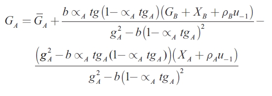
First, the model is analyzed for region A when it treats its exports as given. Following Gramlich, in this "quasi-closed" economy, governments are sophisticated enough to know that imports are endogenous, but not sophisticated enough to know that exports are, too. In this case, the sub-national authority is assumed to solve its model for y and dD and then to set the loss-minimizing value of government spending. The solution for the best-response function of one region, when the local level of expenditure of the other region is taken as exogenous is given by:
 | [8] |
Where  is the normal level f expenditure, which depends positively on
  A and negatively on
  and r; and gA is the government spending multiplier for region A. These equations are given by the following expressions:
 | [9] |
 | [10] |
Where mA is the import propensity of region A. In order to simplify the presentation, in the following equations the coefficient of shocks exhibited in region A is represented by βA ,while the coefficient of shocks presented in region B is represented by βb. In the case of the normal level of expenditure, G, the coefficients of y are represented by δ and the coefficients of (D+rD) by φ . The superscripts characterize the model under analysis4. Taking into account this nomenclature, equations (8) and (9) now become:
 | [11] |
 | [12] |
In this model, the stabilization strategy for the fiscal authority is different when the shock occurs in the same region and when it occurs in the other region. In the case of shocks in region A, the coefficient for  is equal to -1, when there is no consumption loss from rising debt levels (b=0). Thus, the optimal policy for region A should be that of completely offsetting the movements in XA or u with countervailing movements in GA. In this case, the loss value would be zero. When b>0, the local government must balance marginal costs and benefits from stabilization, and it will correct only part of it. The coefficient of
  is now between 0 and 1, declining as b increases. This means that the coefficient response is higher when the debt is incurred by the central government than when the debt is assumed by local authorities.
It is interesting to note that the fiscal response coefficients are lower in the presence of intergovernmental transfers than in the case considered by Gramlich, where local authorities collect their own taxes. The response increases as αA increases. In the extreme case when αA is equal to one, these coefficients are equal in both situations. Unlike the case where local governments are responsible for collecting their own taxes, the presence of transfers makes the optimal level of expenditure in region A dependent on the expenditure and shocks presented in the other region.
This is because the revenue of region A (transfers) depends on the real output of both regions (yA + yB), which in turn affecs fiscal policy.
Whenever shocks occur in region B, the coefficient for  is equal to zero, where b is equal to zero. Thus, when there is no consumption loss from increasing debt, the optimal strategy policy for region A is to do nothing. Nevertheless, when b is greater than zero, the coefficient is positive and increases as b increases. Therefore, when regions consider imports as endogenous but exports as exogenous, a positive shock in region B will have positive spillovers in region A. This happens because the increase in aggregate demand allows for higher taxes and, through this mechanism, a larger level of transfers. This can be viewed as a local government internalizing the benefits provided to residents of other jurisdictions and using them for their own local fiscal decisions. In the different situations analyzed, whenever the serial correlation coefficient is zero, shocks will not persist and it will not be possible for the authority to counteract with a stabilization strategy. The response values would rise as ρ rises.
The Model with Endogenous Exports
The second model analyses the case of a government which knows that imports and exports are endogenous, and as a result of this situation an expansionary fiscal policy in region B will affect exports and domestic income in region A. When subnational authorities consider this in their own stabilization strategy, it is necessary to solve the system simultaneously for both regions. The solution assumes that the authority of region A takes the government spending of region B as exogenous, as in the Cournot-Nash solution. The solution now becomes:
 | [13] |
The normal level of expenditure is:
 | [14] |
As in the previous model, represents the normal level of expenditure. This variable depends on the economic behavior in the same region; it is positively related to the real output target level, and negatively related to the stock of the debt and the real interest rate. In contrast to when exports are exogenous, the level of expenditure is also affected by parameters of region B. In particular, when both regions are symmetric in variables and parameters, the optimal level of expenditure is larger when exports are exogenous than when exports are endogenous. This is because the presence of trade interactions between regions makes the coefficient of yA lower in the second case.
Moreover, when trade interactions between regions are considered, shocks of region A and B have negative coefficient responses. This means that when the fiscal authority of region A has a model for its own region and for region B and solves them simultaneously, it can offset movements in uA , uB and GB with movements in GA The optimal strategy for the sub-national government depends on balancing present output gains and future consumption losses with trade interactions. Finally, the presence of intergovernmental transfers means that fiscal response coefficients and the normal level of expenditure (in the absence of shocks) are higher than when taxes are collected by the sub-national governments.
Game in A Non-Cooperative Solution
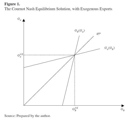
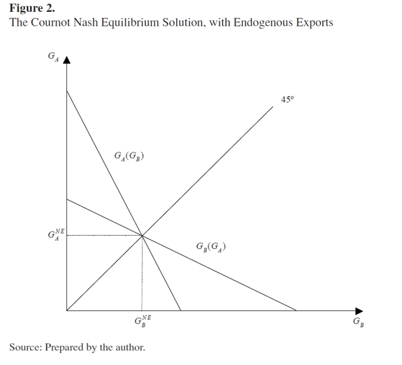
In this section, the Nash equilibrium is estimated for the best-response functions derived above for both the model with exogenous exports and the model with endogenous exports. The solution implies that movements in the output target level and in the fiscal policy in region B would affect not only the optimal stabilization strategy to respond to shocks in region A, but also its normal level of expenditure. To examine the Nash equilibrium solution, region A's best responses are given in equations (8) and (11). In both cases, the best response for region B is found by analogy and corresponds to the reflection around the 45° line of the bestresponse function of region A. Combining the best responses, as in Figure 1 and 2, the Nash equilibrium solution is obtained for the different cases.
The Model with Exogenous Exports
In this section, it is assumed that exports are exogenous , there exists a unique Nash equilibrium, and the government expenditure equilibrium is given as follows:
 | [15] |
The Nash equilibrium for the model is illustrated in Figure 1. It is important to note that when trade interactions are not considered, the best-response functions for region A and for region B are upward-sloping, since the coefficient of the expenditure of the other region has a positive sign. When there are no shocks, the optimal level of expenditure is given by  , which now depends on the economic performance of both regions, positively on
  , and negativly on DA, DB and the real interest rate. The normal level of expenditure is represented by the following equation:
 | [1] |
The second term in equation (15) reflects the response coefficient to a shock in region A. The optimal stabilization strategy is negative and depends on the balancing of present output gains and future consumption losses. This means that the sub-national authority must balance marginal cost and benefits and it will generally correct only part of the stabilization deficiency. The third term reflects the response coefficient to shocks in region B. As before, this response coefficient is positive, which means that when the trade interactions are not considered, a positive shock in region B will have positive spillovers in region A. Thus, there is an interdependence of expenditure determination between regions, due to the fact that an increase in the level of spending in region B raises optimal expenditure in region A5.
In the symmetric case, when the output target level, the stock of the debt and parameters b, m and α are equal in both regions, the government expenditure is lower at the Nash equilibrium when the model is solved using transfers from the central government as compared to the case when they are not used. For region A, this difference decreases as the percentage of transfers to this region, α , increases.
In a decentralized framework, when different interactions between regions are considered, the fact that transfers are determined as a proportion of income taxes has important implications for sub-national finances and for the overall finances of the country. One of the implications is that the pro-cyclical character of the income of the country will affect the level of transfers to the sub-national governments. For instance, when the economy is in boom and regions receive more revenue, the level of expenditure grows more than necessary, and when the economy is in recession, priority public spending can be affected (see for example Cassette & Paty, 2010; Prud'Homme, 1995; Tanzi, 1996; Weingast, 2009).
The Model with Endogenous Exports
When the sub-national authorities are sophisticated enough to consider that exports are endogenous, the Nash equilibrium solution for the symmetric case6 is given by:
 | [17] |
The Nash equilibrium for the model with endogenous exports is illustrated in Figure 2. As explained, when trade interactions are taken into account, the coefficient of the government expenditure of the other region has a negative sign, implying that the best response functions for region A and region B are downward- sloping.
According to the response coefficients to shocks, the Nash equilibrium solution of this model indicates that the fiscal authority in region A can offset shocks in both regions by movements in its level of expenditure, since both coefficients are negative. The optimal strategy in each case will depend on parameters b, m and α in both regions. In the Nash equilibrium, the normal level of expenditure in region A depends on the economic behavior of both regions. Nevertheless, in contrast to when exports are exogenous, the connection between jurisdictions is explained not only by transfers but also by trade interactions between regions. The following equation reflects the behavior expenditure when both regions are symmetric in their parameters.
 | [18] |
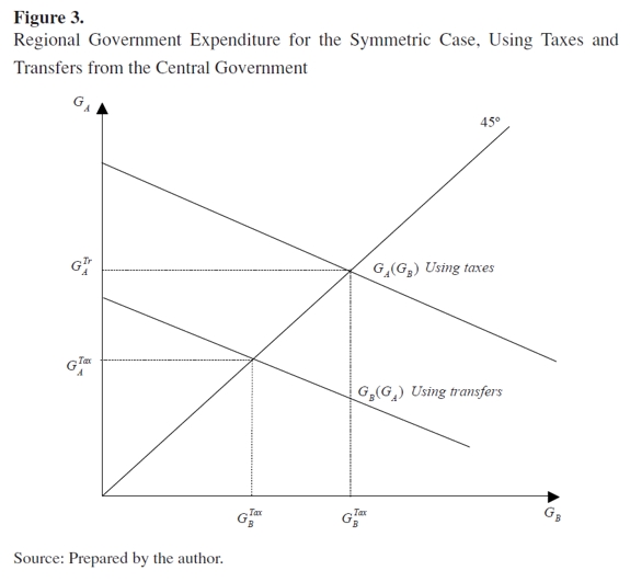
In comparison to when exports are exogenous, the level of expenditure in this model is the lowest for regions A and B. However, this level is highly sensitive to the differences in the marginal propensity to import. As shown in Figure 3, expenditure at the Nash equilibrium solution is higher when taxes are collected by local authorities than when regions receive transfers from the central government. In both cases the loci are downward-sloping, implying that when authorities in region B increase expenditure, the best response for region A, in order to minimize the loss function , is to reduce its own level of spending. The difference between the level of expenditure by using taxes (GTax) and by using transfers (GTr) becomes smaller as the percentage of transfers to this region a increases.
Cooperative Equilibrium
In this section, it is assumed that the central government engages in national cooperation, coordinating the policies of regions in order to achieve the minimum consumption loss in the country, which is obtained by adding the loss function of region A and region B as follows:
| L = LA + LB | [19] |
In this model, the central government sets GA and GB in order to minimize the loss function of the country, subject to the economic model of both regions. This condition allows the central government to internalize the benefits or costs of externalities from one local jurisdiction to another . Comparing the non-cooperative game presented in the section above with the model of cooperative equilibrium presented here allows us to determine in which fiscal structure the response to shocks and expenditure is greater.
Decentralization might involve the distribution of revenue assignments and expenditure responsibilities across different tiers of the public sector. From the perspective of expenditure assignment, each function should be assigned to the lowest level of government consistent with its efficient performance. In principle, the central government should provide public services in the cases where there are differences in demand, there are large spillovers between jurisdictions, and the additional cost of local administration outweighs its advantages. Therefore, local governments have responsibility for those public activities for which spillovers are limited or absent (Bird, 1993). One issue that is addressed here is whether the overall size of the government is greater when the local authority has autonomy to determine the level of expenditure, or when the central government has control over these decisions.
Brennan and Buchanan (1980) maintain that decentralization can serve as a constraint on unwanted government expansion. They contend that fiscal competition can exert some disciplinary force. According to this argument, we should expect to find that the size of the government sector is inversely proportional to the extent of fiscal decentralization. Nevertheless, the empirical evidence concerning this is not conclusive (see for example Jin & Zou, 2002; De Mello, 2000; Oates, 1990). Additionally, the experience of some Latin American countries has shown that overall public spending rises during the first stages of a decentralization process, with important macroeconomic consequences for the countries (see Fukasaku & De Mello 1998; Garman et al., 2001; González, 2008; Ter-Minassian, 1997). The models that are considered here allow us to determine under which conditions the level of expenditure, and consequently the size of the government, is larger.
As in the analysis presented for the non-cooperative solution, here the model is solved for two cases. In the first case, local governments of region A and B assume exports are exogenous. In the second, the authorities of both regions understand that exports of region A correspond to imports of region B and vice versa, with consequences for the domestic income and fiscal variables.
Benevolent Central Government with Exogenous Exports
In this case, it is assumed that sub-national governments are able to cooperate directly, which is equivalent to assuming a benevolent central government. Now the solution is as follows:
 | [20] |
In the cooperative solution, the optimal strategy to respond to shocks observed in the same region has a negative sign, implying that the sub-national authority can offset those shocks by movements in GA, while the optimal strategy to respond to shocks in the other region has a positive sign. The signs of the response coefficient to shocks are similar to the Nash equilibrium solution in the non-cooperative game. However, the optimal stabilization strategy in each case depends on the trade interactions presented in each region. Again as b rises, the response coefficient falls because stabilization needs are balanced against debt reduction needs. The normal level of expenditure is given by the following equation:
 | [21] |
When national co-operation is engaged in order to minimize the loss function for the country , the normal level of expenditure is higher than in the Nash equilibrium case.
The Model with Endogenous Exports
The optimal fiscal strategy to respond to shocks and the normal level of expenditure when governments are sophisticated enough to understand that both exports and imports are endogenous is given by:
 | [22] |
 | [23] |
When the model is solved simultaneously assuming that authorities recognize that the exports of region A are imports of region B, the optimal solution for the public expenditure is higher in the cooperative policy game as compared to the noncooperative solution, when both regions are symmetric. This is because of positive spillovers. In fact, because prices are fixed, an increase in GA raises  A, which in turn increases the total tax revenue, implying that more transfers go to region B, and that resulting losses in consumption are thereby reduced.
This situation is shown in Figure 4, where GNC represents the Nash equilibrium in the non-cooperative model and GC represents the cooperative solution. In the symmetric case, the schedule for the non-cooperative solution is flatter than for the central government solution, since the response coefficient in the first model is smaller in relation to the second model.
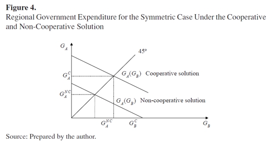
For the symmetric case, it can be concluded that the government is smaller in the non-cooperative solution than in the cooperative solution. This finding supports Brennan and Buchanan's (1980) decentralization hypothesis. However, when asymmetries among regions are observed, this conclusion could be different. In the next section, asymmetric cases when the level of expenditure is lower under the cooperative solution are analyzed using numerical simulations.
NUMERICAL SIMULATIONS
In order to explain the differences between the models presented above when asymmetries across regions are observed, numeral simulations of the optimal strategy for the government to respond to shocks and for the normal level of government expenditure are presented in Tables 1, 2 and 3. In order to carry out this analysis, Gramlich's model was estimated for the non-cooperative game and for the cooperative solution. This allows us to compare the effect on the optimal level of expenditure when transfers are used, compared to the case where regions have autonomy to collect taxes by applying a game approach.
Simulations of Tables 1, and 2 consider different scenarios, depending on the parameters of the models: i) b, how the jurisdiction balances the loss of output due to demand or supply shocks with any stabilization policy debt incurred when responding to these shocks; ii) import and export propensities, (mA and mB); and iii) the percentage of income taxes that the central government distributes to the regions (αA and αB). With respect to transfers, two different situations are considered. First, it is assumed that transfers are evenly distributed among regions of the country, which means that αA = αB (cases from A to D). The second case assumes that transfers are distributed according to the size of the region, and the percentage of the revenues is calculated taking into account the home spending of the region (1 - m) (cases from E to I).
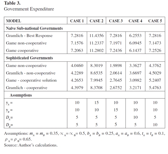
Table 3 presents simulations for the normal level of expenditure, considering changes in the output target level and the stock of the local public debt in both regions. In all cases, it is assumed that the marginal propensity to consume (a) and the tax rate (t) are the same in both regions. Additionally, it is assumed that the central government establishes the tax rate and collects taxes for the country.
When changes in parameters of regions are considered, the simulations yield a number of interesting results. First, in all models, the response coefficients and the normal level of expenditure are higher when the debt is incurred by the central government and the value-added share (b) is smaller, as opposed to the case in which the sub-national authorities assume the debt. Second, for all cases, whenever governments recognize that exports are endogenous, the response coefficients for demand shocks of regions A and B have a negative sign and consequently subnational authorities can offset them by movements in the level of expenditure.
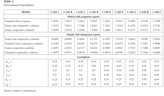
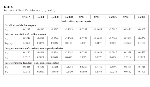
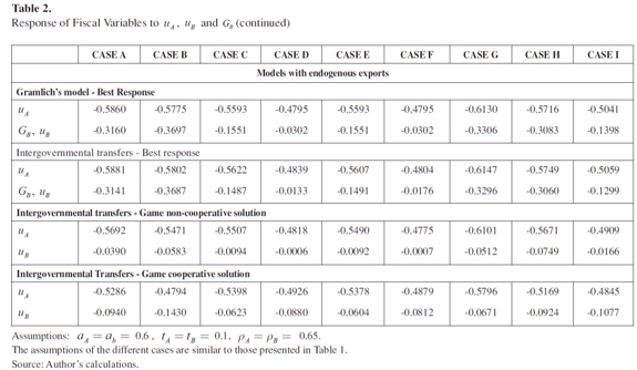
Therefore, when governments are naive, a positive shock in region B has positive spillovers in region A.
In particular, when transfers are evenly distributed among regions (αA = α B = 0.5), there is a more volatile response in models with endogenous exports, taking values from 4.0096 to 9.0788, compared to models with exogenous exports, where the response only varies between 7.1576 and 7.9517. Additionally, when simulations are carried out under assumptions of sophisticated governments and DA = DB, having yA greater than yB produces the highest response among the different scenarios. On the other hand, when yA is lower than yB , this produces the lowest response. For example, in the game with a non-cooperative solution, the responses are 8.3019 and 1.9898 respectively.
Thirdly, when the model is solved for one region, the best-response function for optimal government expenditure that minimizes the loss function of region A is higher when governments are autonomous to collect their own taxes compared to the model that assumes the presence of transfers from the central government. This result takes place despite the positive spillovers of region B and can be explained because the response coefficient to a shock in region A is higher in Gramlich's model due to the absence of α.
Nevertheless, when the marginal propensity to import in region A is lower than in region B, the optimal level of expenditure in the absence of shocks is higher when there are intergovernmental transfers than when they are not used. This suggests that when the central government collects taxes and redistributes them across regions, the level of expenditure for regions with relative low marginal propensity to import is higher than when each region collects its own taxes. This in turn implies that regions with low propensity to import can internalize benefits from the other region, such as an expansionary policy or a higher domestic income. The precise relationship between these models depends on the import and export propensities in both regions.
Another interesting finding is that the level of expenditure is higher when the central government coordinates fiscal policy, as opposed to when sub-national authorities have autonomy to carry out their own policies. This result is valid in all cases, except when parameter b is higher in region A than in region B and the central government assumes the sub-national public debt. The difference in the level of expenditure between these two models grows as the difference between bAand bB increases. This means that for large regions with high value-added share, the level of expenditure is lower in the presence of coordination than when there is no coordination among regions.
The previous results support the assertion that government is smaller in a decentralized structure where each region minimizes its own loss function, as opposed to the case when the central government coordinates the policies in order to minimize the loss function of the whole country. The exception to this is when the share of the national interest burden incurred by tax-payers in region A is greater than in region B. Thus, when there are differences in the size of regions and the central government assumes the sub-national debt, the level of expenditure will be lower if the central government coordinates policies across regions. This conclusion is not valid when local authorities assume the debt; in this case the government is always smaller under non-cooperative models.
Table 3 shows the main findings of the simulations when changes in the optimal level of output and in the stock of the debt are observed. In order to carry out these simulations, it is assumed that parameters a, t, m, b and α are symmetric in both regions. In addition, a benchmark case is established for variables y and D, in which yA=yB and DA=DB. The simulations are carried out by changing one of these variables.
It can be observed from the results of the simulations that when each sub-national authority behaves in the Nash manner, choosing its own level of expenditure to minimize the loss consumption function, the best response function for each region is not affected by changes in output or in the stock of the debt of the other region. The most important implication of Table 3 is that there is not a unique pattern to determine whether the expenditure is higher in a non-cooperative or in a cooperative model. This situation depends on the economic conditions of both regions. In particular, the result is affected by the differences in y and D across regions. The level of expenditure in region A is lower using a non-cooperative approach when y and D are similar in both regions and when these variables are higher in region B. In contrast, G is lower in the cooperative solution when the output and the stock of debt are higher in region A.
According to these results, it is not possible to generalize that governments are smaller in decentralization contexts. In fact, according to the simulations, this would depend on the relationship between b, y and D in both regions. This conclusion supports the results of some empirical studies. In particular, Oates (1990), in his review of the literature, found evidence in some studies that as the degree of decentralization increases, the size of the government decreases, and evidence in other studies for the opposite. Based on empirical evidence, this author also suggests that decentralization itself does not constrain the government size, and that if a smaller government is the aim, other measures are probably in order. Recently, Cassette and Paty's (2010) empirical study for European countries found that, in the long run, decentralization reduces central expenditure, but increases sub-national public expenditure and aggregate public expenditure. Additionally, as Jin and Zou (2002) found by carrying out an econometric analysis using panel data from 32 industrial and developing countries for the period 1980-1994, when expenditure is decentralized, national governments become smaller, and subnational governments as well as aggregate governments increase in size.
CONCLUSIONS
This paper presents a comparative analysis of the fiscal response to shocks and the level of expenditure in the sub-national public sector in non-cooperative and cooperative models. The analysis is undertaken by using, on the one hand, models that assume that central governments collect taxes of the whole country and redistribute them across regions and, on the other hand, models that assume that sub-national income comes from the collection of regional taxes, as in Gramlich (1987).
There is an assumption that governments tend to spend more when acting in non-cooperative models. However, as Brennan and Buchanan (1980) have suggested, decentralization can also serve as a constraint on the expansion of government expenditure. The analysis presented in this article serves to illustrate that, even within a highly simplified model, it is not possible to conclude whether subnational governments operating in a non-cooperative national environment will spend more or less than in a cooperative solution, where the central government coordinates policies in order to minimize the loss function of the country. The result will depend on the economic conditions of the regions and on the trade interactions between them. In particular, it was found that when the central government assumes sub-national debts and the share of the national interest burden incurred by tax-payers in region A is greater than in region B, the level of the expenditure is lower under a cooperative model. Similarly, this result is valid when the output target level and the stock of the debt are higher in region A. These results are consistent with empirical studies that have not found clear evidence on which fiscal structure results in smaller government size.
The results also suggest that the response coefficients for demand shocks differ when there are large differences in the trade interactions among regions. In fact, when parameters are similar across regions, this response is higher under the noncooperative solution, while in the presence of differences in the marginal propensity to import, the response coefficient is higher when the central government coordinates fiscal policies of regions.
FOOTNOTES
1 For details on the process of decentralization in Latin America see Escobar-Lemmon (2001), Falleti (2005), Falleti (2006), and Garman, Haggard, and Willis (2001).
2 Details of the Colombian decentralization process can be found in Bonet, Pérez, and Ayala (2014), Iregui, Ramos, and Saavedra (2001), Lozano, Ramos, and Rincón (2007), Melo (2002), and Zapata, Acosta, and Gonzalez (2001).
3 Prices are assumed to be fixed in order to conduct a comparative analysis with Gramlich models. An interesting analysis for future research would be to consider prices changing over time.
4 BR stands for best response models, ExE for models with exogenous exports, EnE for models with endogenous exports, NC for non-co-operative solution models and C for cooperative models.
5 The analysis is compared to the income determination in the Mundell-Fleming two-country model, with fixed exchange rates, in which an increase in the home country income increases foreign output.
6 The analysis when the parameters vary between regions is presented in the next section by using numerical simulations.
REFERENCES
[1] Bahl, R., & Bird, R. (2008). Subnational taxes in developing countries: The way forward. Public Budgeting & Finance, 28(4), 1-25. [ Links ]
[2] Bahl, R., & Linn, J. (1994). Fiscal decentralization and intergovernmental transfers in less developed countries. The Journal of Fiscal Federalism, 24, 1-19. [ Links ]
[3] Bird, R. (1993). Threading the fiscal labyrinth: Some issues in fiscal decentralization. National Tax Journal, 46(2), 207-227. [ Links ]
[4] Bonet, J., Pérez, G., & Ayala, J. (2014). Contexto histórico y evolución del SGP en Colombia (Documento de Trabajo sobre Economía Regional 205). Banco de la República, Sucursal Cartagena. [ Links ]
[5] Brennan, G., & Buchanan, J. (1980). The power to tax: Analytical foundations of a fiscal constitution. New York: Cambridge University Press. [ Links ]
[6] Cassette, A., & Paty, S. (2010). Fiscal decentralization and the size of government: A European country empirical analysis. Public Choice, 143(1-2), 173-189. [ Links ]
[7] Escobar-Lemmon, M. (2001). Fiscal decentralization and federalism in Latin America. Publius: The Journal of Federalism, 31(4), 23-41. [ Links ]
[8] Faguet, J. (2014). Decentralization and governance. World Development, 53, 2-13. [ Links ]
[9] Falleti, T. (2005). A sequential theory of decentralization: Latin American cases in comparative perspective. American Political Science Review, 99(3), 327-346. [ Links ]
[10] Falleti, T. (2006). Una teoría secuencial de la descentralización: Argentina y Colombia en perspectiva comparada. Desarrollo Económico, 46(183), 317-352. [ Links ]
[11] Feltenstein, A., & Iwata, S. (2005). Decentralization and macroeconomic performance in China: Regional autonomy has its costs. Journal of Development Economics, 76(2), 481-501. [ Links ]
[12] Fukasaku, K., & De Mello, L. (1998). Fiscal decentralization and macroeconomic stability: The experience of large developing and transition economies. In Fukasaku K. & Hausmann R. (Eds.), Democracy, decentralization and deficits in Latin America. Paris: OECD. [ Links ]
[13] Garman, C., Haggard, S., & Willis, E. (2001). Fiscal decentralization: A political theory with Latin American cases. World Politics, 53(2), 205-236. [ Links ]
[14] González, L. (2008). Political power, fiscal crises, and decentralization in Latin America: Federal countries in comparative perspective (and some contrasts with unitary cases). Publius: The Journal of Federalism, 38(2), 211-247. [ Links ]
[15] Gramlich, E. (1987). Sub-national fiscal policy. In J. M. Quigley (Ed.), Perspectives on local public finance and public policy (vol. 3, pp. 3-27). London: JAI Press. [ Links ]
[16] Iregui, A. M., Ramos, J., & Saavedra, L. A. (2001). Análisis de la descentralización fiscal en Colombia. Banco de la República, Subgerencia de Estudios Económicos. [ Links ]
[17] Jin, J., & Zou, H. (2002). How does fiscal decentralization affect aggregate, national, and subnational government size? Journal of Urban Economics, 52(2), 270-293. [ Links ]
[18] Lozano, I., Ramos, J., & Rincon, H. (2007). Implicaciones fiscales y sectoriales de la reforma a las transferencias territoriales en Colombia (Borradores de Economía 437). Banco de la República. [ Links ]
[19] Melo, L. (2002). The flypaper effect under different institutional contexts: The Colombian case. Public Choice, 111(3-4), 317-345. [ Links ]
[20] De Mello, L. (2000). Fiscal decentralization and intergovernmental fiscal relations: A cross-country analysis. World Development, 28(2), 365-380. [ Links ]
[21] Oates, W. (1990). Fiscal federalism: Overview. R. Prud'Homme, Public finance with several levels of government. Brussels: Foundation Journal Public Finance. [ Links ]
[22] Oates, W. (2005). Toward a second-generation theory of fiscal federalism. International Tax and Public Finance, 12(4), 349-373. [ Links ]
[23] Prud'Homme, R. (1995). The dangers of decentralization. The World Bank Research Observer, 10(2), 201-220. [ Links ]
[24] Rodden, J. (2004). Comparative federalism and decentralization: On meaning and measurement. Comparative Politics, 36(4), 481-500. [ Links ]
[25] Shah, A. (2004). Fiscal decentralization in developing and transition economies: progress, problems, and the promise (Working Paper 3282). World Bank Policy Research. [ Links ]
[26] Tanzi, V. (1996). Fiscal federalism and decentralization: A review of some efficiency and macroeconomic aspects. In Annual World Bank conference on development economics, pp. 295-316. [ Links ]
[27] Ter-Minassian, M. T. (1997). Decentralization and macroeconomic management (EPub 155). International Monetary Fund. [ Links ]
[28] Weingast, B. (2009). Second generation fiscal federalism: The implications of fiscal incentives. Journal of Urban Economics, 65(3), 279-293. [ Links ]
[29] Zapata, J. G., Acosta, O. L., & González, A. (2001). Evaluación de la descentralización municipal en Colombia. ¿Se consolidó la sostenibilidad fiscal en los municipios colombianos durante los años noventa? Archivos de Economía, Departamento Nacional de Planeación. [ Links ]


