English (pdf)
 Article in xml format
 Article references
 Send this article by e-mail
 Cited by SciELO
  Cited by Google
  Similars in
SciELO
Similars in
SciELO  Similars in Google
 Permalink
INTRODUCTION
In 1958 Modigliani and Miller posited that in the absence of taxes capital structure is irrelevant for firm value. The traditional textbook formula for the Weighted Average Cost of Capital (WACC) includes tax savings in a factor (1-T) within the formula as follows:

where the WACC is the weighted average cost of capital, Kdt is the cost of debt, T is the corporate tax rate, D% and E% are the weights of debt and equity based on firm market value, and t-1 and Ket is the cost of levered equity. The firm market value is understood as the present value of Free Cash Flow (FCF) at the WACC.
This paper develops a procedure for properly calculating TS, including the case where Losses Carried Forward (LCF) are allowed and where there is (non-operational) OI. This is important because the value of TS can be a substantial part of value.
The paper consists of the following sections: Section One reviews the existing literature on the calculation of TS and its market value. Section 2 deals with what TS are and explains how they are created. Section 3 examines several cases of levered and unlevered firms and identifies the conditions necessary for totally or partially earning TS. Finally, Section 3 illustrates the conditions that render the textbook formula for the WACC a very special case.
LITERATURE REVIEW
TS are important because, as Fama and French (1998) put it, "good estimates of how the tax treatment of dividends and debt affects the cost of capital and firm value are a high priority for research in corporate finance" (p. 819). In the same vein, Kemsley and Nissim (2002) estimate that the value for debt TS is approximately as high as 40 percent of debt balance and 10 percent of firm value, net of the personal tax disadvantage of debt. Graham (2000) shows that firms derive significant tax savings from debt, estimated at 9.7% of firm value. Graham and Lemmon (1998) calculated the figure as 11%, Graham (2003) as between 7.7% and 9.8% and Korteweg (2010) as 5.5%. Van Binsbergen, Graham and Yang (2010) determined that on average the value of the tax benefits of debt represents 3.5% of the book value of assets. A similar measure for a group of Colombian traded firms between 2001 to 2010 gives a range of values for TS as a percentage of total firm market value between 5.4% and 9.3%, depending on the discount rate used to estimate the value of TS, see Gutiérrez-Ruiz, Salas-Pérez and Vélez-Pareja (2011); note that, when calculating the size of TS in this case, the authors used the algorithm used in this paper.
This current of the literature is intended to calculate the value of tax savings. However, less effort has been expended in examining how the tax savings are calculated. Most authors and textbooks calculate TS using only the interest payments. The general approach used is to multiply the T by interest payments. That is, the implicit assumption is that the only source of TS is interest payments and that there is always enough operational profit to generate tax savings: see, for example, Arditti and Lévy (1977), Gonedes (1981), Masulis (1983), MacKie-Mason (1990), Arzac (1996) and Liu (2009).
Firms obtain financial tax benefits from sources other than interest expenses and in some cases do not obtain those benefits in the year they pay taxes. For instance, see Dammon & Senbet (1998), Graham (2000) and Grabowski (2009).
Graham (2000), recognizes that "each marginal tax rate incorporates the effects of non-debt tax shields, tax-loss carrybacks, carry forwards, tax credits, the alternative minimum tax, and the probability that interest tax shields will be used in a given year" (p. 1902). Grabowski (2009) asks if firms deduct interest expenses at the statutory T or not. He answers in the affirmative and goes on to argue that, "... many companies do not expect to pay the highest marginal rate for long periods of time. Because of tax loss carry-backs and carry-forwards and the cyclical nature of some industries, a substantial number of companies can expect a very low tax rate" (p. 38).
Some readers might consider that the idea of not being "able to utilize all their interest deductions fully because of [...] insufficient taxable income" (Cordes & Sheffrin, 1983, p. 95) is just an academic straw man. It is not. It is real, and some papers report the situation, seeking to estimate the effective tax value associated with interest expenses. See, for example, Newbould, Chatfield and Anderson (1992) who say explicitly that, "the ability to use tax shields each year is forecast and excess shields are rolled forward until they can be used" (p. 53).
Molnár and Nyborg (2013) adjust the WACC when leverage is constant. They do not deal with the proper calculation of TS, continuing to assume that TS = Interest χ FE and using the (1-T) factor. This recent paper deals with a different context, examining how personal taxes affect the value of TS and, hence, the optimal capital structure under trade-off theory. On the other hand, Koziol (2014) deals with "the possibility of a default, as the main characteristics such as the default probability and potential bankruptcy costs are commonly disregarded. This paper aims at providing a tractable extension of the well-known WACC approach for both default risk and bankruptcy costs". Citing several authors in their support, Pierru and Atallah (2013) develop a mathematical model for scheduling debt in such a way that TS are maximized: "This result is new since the literature on tax shields valuation -including recent contributions by Fernandez (2004), Arzac and Glosten (2005), Cooper and Nyborg (2007), Grinblatt and Liu (2008), Liu (2009) and Qi (2011)- has never specifically considered the case of multinational firms" (p. 1).
Barbi (2012) approaches the problem of determining the value of the TS by defining its value using a risk-neutral probability approach. Tham and Wonder (2001, 2002) use the same approach to define the discount rate for TS in order to estimate value.
Analysts are interested in counting with a procedure for calculating TS when forecasting financial statements and cash flows in order to estimate firm and equity values. This problem is examined in Section Three.
WHAT ARE TAX SHIELDS?
Because cash flows are discounted using a discount rate that takes into account the sources of financing (debt and equity) this paper introduces the effect of tax savings on the WACC. For this reason it is particularly interesting to focus on FE.
FE are defined as a general concept rather than as interest charges because, depending on a given country's tax law, they may comprise interest, banking commissions, foreign exchange losses, capital stock adjustments when inflation adjustments are made to financial statements or even, as in Brazil, interest on equity capital (see, Vélez-Pareja & Benavides-Franco, 2011 and Vélez-Pareja & Tham, 2010). As has been seen, some TS do not originate from interest expenses and others are not reflected in the traditional formula for the WACC (eq. 1). Thus, the traditional formula might underestimate the cost of capital and, as a consequence, overestimate firm value. Gilson, Hotchkiss and Ruback (2000) recognize this fact: "Capital cash flows measure the cash available to all holders of capital and include the benefit of interest and other tax shields" (p. 49) (emphasis added). See also Kemsley and Nissim (2002).
As this article will demonstrate, TS mean that the effect of any additional expense on the bottom line (i.e. net income) is reduced. Given certain conditions, an after tax expense Eat becomes Ebt χ (1-T) and hence, TS are Ebt x T.

In other words, the subsidy firms receive from the government is

SPECIAL AND TYPICAL CASES: A SIMPLE PROCEDURE FOR CALCULATING TAX SHIELDS
On occasion, firms are not able to earn all the potentially available TS. The reader will easily identify situations where the conditions presented above are not met -such as start-ups or firms in financial distress. In such circumstances it is necessary to consider EBITAdj:
Consider three situations:
EBITAdj, is Earnings before Interest and Taxes, EBIT + OI - Other Expenses excluding FE. This EBITAdj is the amount offset against FE when calculating Earnings before Taxes (EBT).
The question is whether it makes any difference. It does. Before moving forward, consider the following assertion: The "right" to earn TS is based on the results of the income statement which itself is based on accruals that do not imply a cash flow. This means that TS are based on accounting figures. In fact, anyone could verify that taxes are calculated on the basis of accounting results that imply accruals. As can be seen from income statements, the "right" to the TS depends on EBITAdj. TS are a strange mix of accounting and accrual related to the WACC, which rely on market values.
A summary of these ideas follows. Table 1a illustrates the case when EBITAdj ≥ FE.
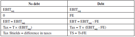
In this case the TS are equal to FE x the T. In this case, the traditional textbook formula works.
Examine the textbook formula for the WACC in (1) and note that it only applies to case 1. That is, when EBITAdj ≥ FE, taxes are paid in the same period, when interest payments are the only source of TS.
Proposition 1. When EBITAdj ≥ FE, TS are equal to the corporate T multiplied by FE (T χ FE).
Table 1b, shows the TS calculations for cases where EBITAdj is non-negative and less than FE.
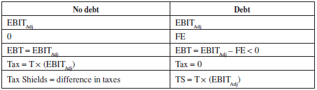
This second case shows that TS are not equivalent simply to T x FE, as predicted by eq. (2b), but T x EBITAdj. Observe that even if a firm does not pay taxes (as in Table 1b) TS are earned. This happens because EBITAdj exists to offset the FE.
This may be explained (see Table 1b) as the difference between T x EBITAdj (when the firm pays taxes and has no debt) and 0, when the firm does not pay taxes because EBITAdj < FE.
Proposition 2. When 0 ≤ EBITAdj< FE, TS are not equal to T χ FE. As Table 1b shows, in this case, TS are T χ EBITAdj.
Table 1c. illustrates the case when EBITAdj < 0.
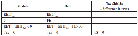
This third case shows that when EBITAdj is negative, the TS are zero.
Proposition 3. When EBITAdj < 0, there TS are not earned.
Practitioners and some academics consider it to be a rule that if a firm has losses, then TS are not earned. This is not true. A firm will enjoy TS if it is subject to income tax, including in cases where, due to losses, it does not pay taxes (as in Table 1b). The condition for the existence of TS is that the firm must pay income tax and the EBITAdj is non-negative.
In summary, the three situations may be condensed in a step-wise function
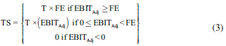
In equation (3) T is not required to be constant. In fact, the equation holds for every period, for each of which a different T could be defined. As using spreadsheets when constructing forecasted financial statements is standard, T can easily be changed in the forecasting horizon. Hence, it is a matter of defining the T for each period in the forecast as an input variable. This poses no significant problem.
It should be noted that Wrightsman (1978), proposed this idea nearly 40 years ago. Surprisingly, most textbooks and papers assume as a general rule that TS are equivalent to the T multiplied by interest charges. This has implications because the use of the WACC textbook formula is generalized when in fact it is a very special case.
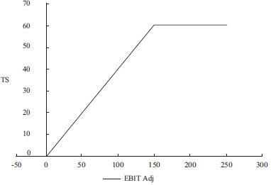
Equation (3) is a segmented function of TS depending on EBITAdj. This is very important because in reality, at least in the early years of new ventures or startups, EBITAdj might be less than FE, or even negative. This means that in those cases it is not always possible to achieve full TS, which might be either zero or less than T χ FE. Only when EBITAdj is smaller than or equal to zero does the firm fail to earn any TS and in this case, the valuation of the cash flow should be carried out using the unlevered cost of equity as the discount rate. This equation (3) is depicted in Figure 1.
Figure 1 shows that when EBITAdj is negative TS is zero, because there is no EBITAdj to offset the FE (first interval, EBITAdj < 0). The second interval, 0 ≤ EBITAdj < Fe, is when there is positive EBITAdj and FE > EBITAdj. This means that part of FE can be offset by EBITAdj and is exactly identical to EBITAdj while the TS is T x EBITAdj. This is the reason why TS is a linear function of EBITAdj: the greater EBITAdj, the greater the TS. The third interval is when FE≤ EBITAdj. This means that no matter how large EBITAdj is, the firm cannot exceed the benefits of TS = T x EBITAdj.
The segmented function for TS may be expressed as
TS = Maximum (T × Minimum (EBITAdj, FE), 0) (4)1
Tables 1a to 1c, and Figure 1, show the relationship between TS and EBITAdj. It can be seen that TS is a function of EBITAdj and hence suffer a risk associated with EBITAdj (a proxy for FCF). For Wrightsman (1978), this is a risky debt; however, the riskiness of TS comes from EBITAdj, not from the debt. With this reasoning, it may be felt that the proper discount rate for TS might be larger than Kd, the cost of debt. Regarding the risk of TS, Brennan and Schwartz (1978) make the following comment, citing the seminal paper of Modigliani and Miller (1963):
This paper is concerned mainly with relaxing the assumption that the tax savings due to debt issuance constitute a "sure stream." Modigliani and Miller [...] acknowledge that "some uncertainty attaches [...] to the tax savings" (1963, n. 5) [...]. They attribute this uncertainty to two causes: first, the possibility of future changes in the tax rate and, second, the possibility that at some future date the firm may have no taxable income against which the interest payments on the debt may be offset. (p. 104). (Our emphasis).
To corroborate the assertion that some practitioners consider that paying no taxes means no TS is earned, see the position of Cooper and Franks (1983). Though their assertion is old, note that it illustrates exactly what many people still think today):
With taxes as the only imperfection, no corporation pays taxes if it issues sufficient corporate debt to make interest charges always equal to taxable income from operations. Interest charges provide a costless alternative mechanism for sheltering taxable income, so alternative tax shield substitutes have no value. The capital budgeting rule requires that all projects should be evaluated on the basis of their pre-tax cash flows, using an unlevered equity required return as the discountrate. (pp. 572-573) (Our emphasis).
The last sentence quoted reflects what many people think: if the firm does not pay taxes (in this case because "interest charges [are] always equal to taxable income from operations") there is no tax benefit capable of affecting the "unlevered equity required return as the discount rate". This is not true, however. If EBITAdj exactly offsets interest charges, then taxable income is zero, but, according to (3), the TS are corporate T multiplied by FE. Hence, the discount rate must include the effect of TS and should not, contrary to what Cooper and Franks (1983) assert, be evaluated using only Ku, the unlevered cost of equity.
Aivazian and Berkowitz (1992) suggest that firms obtain TS when they pay taxes. As seen above, the second segment of equation (3) suggests that, under the circumstances described, firms might not earn enough to pay taxes but may still obtain some TS. When a firm is in this situation it does not pay taxes and yet TS are equal to T χ (EBITAdj).
Miles and Ezzell (1980), consider that TS are uncertain. This is obvious, because as noted above TS depend on forecasts and on EBITAdj. However, it is true that if it is assumed that TS are tax savings that result from interest payments and the textbook formula for the WACC is used, tax savings will be biased.
Now, Tables 2a and 2b show how the (1-T) factor works in the textbook formula for the WACC. If a firm has a loan of $1,000 to be repaid the following year, the T is 40% and taxes are paid in the same year they are accrued, the Cash Flow to Loan (CFL) is shown in the next table.
With T at 40%, TS are $120. In the previous table taxes are paid, and the TS is obtained, in the same year taxes are accrued. In this case, after-tax contractual non capitalized Kd is equal to Kd(1-T) (in this case 30% χ 60% = 18%), which itself is equal to the Internal Rate of Return for the after-tax CFL.
Note that Table 2a includes CFL, which differs from Cash Flow to Debt, (CFD)2. CFL is seen from the point of view of the firm and CFD from the point of view of debt holders.
Table 2a Taxes Paid the Same Yeara. Full TS Coverage
| Year | CFL | TS | After tax CFL |
|---|---|---|---|
| 0 | 1,000 | 1,000 | |
| 1 | -1,300 | 120 | -1,180 |
| IRR** | 30% | 18% |
a In this work, taxes are assumed to be paid the same year are accrued, unless it is said the contrary. This is not a strange situation. Many firms are subject of withholding tax also called a retention tax. This is equivalent to pay taxes the same year as accrued.
* Internal Rate of Return for the loan (from the firm's point of view).
Source: Example and data constructed by the Author.
If taxes are paid during the year after they are accrued, these TS are effectively created when the taxes are paid. In this case, Table 2b shows that when TS appears in the cash flow:
Table 2b Taxes Paid Next Year. TS Fully Earned
| Year | CFL | TS | After tax CFL |
|---|---|---|---|
| 0 | 1,000 | 1,000 | |
| 1 | -1,300 | -1,300 | |
| 2 | 120 | 120 | |
| IRR | 30% | 20% |
Source: Example and data constructed by the Author.
Table 2b shows that, after tax, contractual non capitalized Kd is not equal to Kdt-1(1-T). In this new situation, where taxes are postponed, TS are received the following year, increasing the after-tax cost of debt from 18% to 20%. This is relevant because the trend is to use (1) as a standard and general formula when in fact, it is not. On the contrary, (1) is a very special case for which certain conditions have to be met. These, the conditions for the effect of taxes on the WACC (through the Kd (1-T) expression) are:
Taxes are paid during the same period they are accrued.
EBIT plus OI are greater than or equal to FE and hence, the firm benefits from the full TS.
Interest paid is the only source of TS.
Book value and market value of debt are identical and, furthermore, the market cost of debt is also identical to the contractual non-capitalized cost of debt.
All this means that the traditional textbook formula applies only to very special and unique cases. Notice in Table 2b, as well, that tax savings are received when taxes are paid, not when they are accrued. Moreover, firms can accrue interest payments and delay the payment of taxes until they are due; at is at this point that TS are created, not when interest is paid.
Proposition 4. The textbook WACC formula is valid only when conditions 1 to 4 hold.
This article is illustrated using very simplified typical conditions, but in reality the calculation and the "receipt" of TS can be a little more complex. Down to earth situations such as inflation adjustment to financial statements, losses carried forward, taxes paid in advance or delayed, and exchange rate losses make the calculation of TS difficult, because in the financial model it is necessary to keep control of several conditions at a time and not all of them are reflected in the cost of debt after taxes, Kd × (1-T).
If Losses Carried Forward (LCF) are allowed, TS not created in one period can be recovered in the future when losses are carried forward. Table 3 illustrates the use of LCF.
Table 3 Tax Savings with LCF from Year t to t + 1
| Year t | Yeart+1 | |||
|---|---|---|---|---|
| No debt | With debt | No debt | With debt | |
| EBITAdj | 100 | 100 | 250 | 250 |
| FE | 0 | -150 | 0 | -150 |
| EBT | 100 | -50 | 250 | 100 |
| LCF = Min(-Net Incomet; EBTt+1) | -50 | |||
| Adjusted EBT = EBT + LCF | 100 | -50 | 250 | 50 |
| Taxes 40% | 40 | 0 | 100 | 20 |
| Net Income = EBT - Tax | 60 | -50 | 150 | 80 |
| TS = difference in taxes | 0 | 40 | 0 | 80 |
| TS = Max(T*Min(EBITAdj, FE+LCFt+1-LCFt),0)a | 0 | 40 | 0 | 80 |
| TS from FE | 0 | 60 | 0 | 60 |
| TS from LCF = T*(LCFLev - LCFUnlev) | 0 | 0 | 0 | 20 |
a I am grateful to Mr. Christian Ledig, from SMS Maintenance Services GmbH Duesseldorf. He contributed with helpful comments on this example to make it more general. Source: Example and data constructed by the Author.
Note that the effective T in year t+1 with debt is 20% (20/100) instead of 40% as might be expected. This means that equation (4) is transformed into
TS = Maximum (T × Minimum(EBITAdj, FE + LCFt+1 - LCFt), 0) (5)3
TS =Max(T*Min(EBITAdj,FE + LCFt+1 - LCFt), 0)
Applying equation (5) to the example in table 3 TS is

As shown in Table 3, the TS of 80 consists of 60 from FE (40% χ 150) and 20 from LCF (40% χ 50). Observe that TS are no longer T χ FE. This means that the standard textbook formula for the WACC, equation (1), is no longer valid in cases such as the one shown in Table 3. Notice also that the effect of larger TS in year t + 1 shown in Table 3 is not even captured by the "effective" T. If T (effective) is introduced in (1), the effect is to raise the after-tax cost of debt, instead of lowering it because of greater TS.
Proposition 5. When LCF are allowed and EBIT ≥ FE, Proposition 1 is modified such that TS are the corporate T multiplied by the FE, minus losses carried forward, T χ (FE + LCFt+1 - LCFt) if FE + LCFt+1 - LCFt is not greater than EBITAdj. The upper limit for TS in this case is T χ (EBlTAdj).
It should be stated that current practice defines operational working capital excluding cash and quasi-cash items from the calculation. The net effect of this is that any increase in these items increases Cash Flow to Equity (CFE)4 and FCF5 and the assumption is that all the cash generated is distributed. Hence, if they are not included on the initial balance sheet it is also assumed that the cash flows show no interest income. However, cash and quasi-cash items and their returns do appear in the financial statements, which is inconsistent.
On the other hand, some practitioners subtract interest received from interest paid. This means that CFE and CFD are altered. This makes no sense because, among other things, these are streams of cash from different sources that flow at different rates. Interest received belongs to shareholders and should go to the CFE, and there is no reason to assume CFD should be decreased when netting both interests.
One reason to stick to this practice is the belief that is not necessary to forecast CFE explicitly, when in fact it must be, for several reasons: one is that in reality, it is not usual that firms distribute the total available cash. Another reason is that it is possible to set an input variable in the model that allows the analyst to define the level of desired distribution (the payout ratio). .sing this ratio, it is possible to estimate future dividends, which should make up the essential part of CFE.
That being said, consider the situation of OI, which includes interest income from market securities.
When a firm's OI includes interest income, treating TS as the difference in tax payments distorts the results (see Tables 4a and 4b). Assuming a firm maintains excess cash for future investment, it might finance the new investment partially or totally with internally generated resources and debt. In such a case assume that an unlevered firm has OI (including interest from excess cash) and that when it becomes levered that OI, or a part of it, vanishes and shifts to the payment of interest on debt. This is explained by the fact that if the firm needs debt, the excess cash generated by OI (financial non-operational income) vanishes and hence, interest as OI vanishes as well. This can be explained by considering that, in general, it might make no sense for a firm to keep excess cash invested in market securities and at the same time contract debt at a higher cost. Imagine a firm with excess cash in market securities of 1,000, earning 5%; interest income would be 50. If the firm needs 1,500 for investment it will need to contract a debt of 500 (1,500 - 1,000). If the cost of debt is 10%, interest charges would be 50. The net of interest income and expense disappear and yet it has to pay 50 in interest charges for the new debt. Table 4 shows this. Assume T of 40%, cost of debt 10% and return on cash 4%.
Table 4 Tax Shields When the Firm Has Financial Income (End of Year)
| No Debt | New Debt | With debt | ||
|---|---|---|---|---|
| Year t - 2 | Yeart - 1 | Year t | Yeart+ 1 | |
| Investment | 1.500.0 | |||
| Debt | 0.0 | 500.0 | 500.0 | |
| Excess cash | 1,000.0 | 1,000.0 | 0.0 | 0.0 |
| EBIT | 100.0 | 100.0 | 100.0 | 100.0 |
| OI | 40.0 | 40.0 | 0.0 | |
| EBIT+OI=EBIT4d. Ad) | 100.0 | 140.0 | 140.0 | 100.0 |
| FE | 0.0 | 50.0 | ||
| EBT | 100.0 | 140.0 | 140.0 | 50.0 |
| Tx | 40.0 | 56.0 | 56.0 | 20.0 |
| Tax difference | -16.0 | 0.0 | 36.0 | |
| TS accrued | 0.0 | 0.0 | 20.0 | |
Source: Example and data constructed by the Author.
Applying (4)

Applying eq. (6), with FE not 0

Difference in taxes due is 36. The reconciliation of these two figures is that part of the difference in taxes owed comes from the fact that the levered firm has less OI to be taxed. In this case, less by 40. Consequently it will pay less tax (16 = 40% × 40). On the other hand, the firm has FE of 50. Hence, because in this case EBITAdj is greater than FE, TS is 20 (40% × 50). Note that the difference in taxes is 36, but the TS is 20. It is clear from this example that the difference in taxes due is not always identical to the value of TS.
From the previous example, Proposition 6 emerges as:
Proposition 6. When OI is available, an analysis of levered and unlevered firms that calculates TS to be the difference between taxes due from unlevered and levered firms is distorted. TS have to be calculated as stated in Propositions 1, 2 and 3 and not as the difference in taxes due. Difference in taxes includes the reduction of taxes when funds from OI are used to pay FE.
Proposition 7 is as follows:
Proposition 7. Difference in taxes should be adjusted by -T x (OIunlevered - OI levered).
According to these propositions, the difference in taxes for the previous example (36) has to be adjusted by -40% × 40 = -16. When the difference in taxes is adjusted the correct TS are obtained.
If the textbook formula is a special case, is there a general formulation for the WACC?
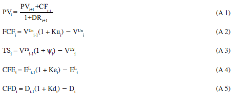
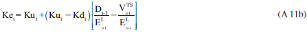
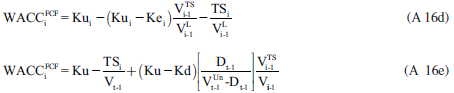
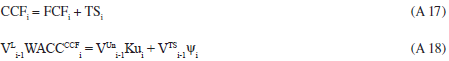
The answer to this question is Yes. There is a general formulation for the WACC. Before proceeding, note that the value of the TS is its present value at a proper discount rate, ψ. Taggart (1991), has studied this issue, presenting the formulas for Kd and Ku as discount rates, but he provides no derivation for them. It can be shown that a general formulation for the WACC for the FCF is (see Tham & Vélez-Pareja, 2002, 2004):
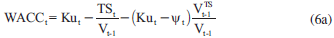
where VTS is the value of TS at ψ and Ku is the cost of unlevered equity; the other variables have been defined previously. When the WACC is written as a function of TS and its value, as in (6a), TS could be earned at any time and from any source that affects the financing of the firm. This seems to be a complex formula, but it greatly facilitates matters when working with the WACC and the FCF, which is required in order to calculate value. For instance, it might be valid for cases where equity capital is adjusted by inflation as in the case of inflation-adjusted financial statements (see Vélez-Pareja & Tham, 2010). It might also apply, as stated above, when a percentage of shareholder dividends is paid as interest on the book value of equity, as in Brazil (see Vélez-Pareja & Benavides-Franco, 2011).
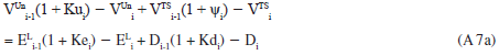
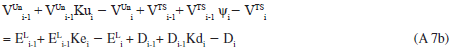
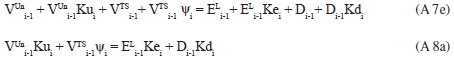
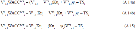
Depending on the assumptions made regarding the risk (discount rate) of TS ψ, the expression for the WACC is more or less complicated. (See Appendix for a derivation of formulas for Capital Cash Flow, FCF, and Equity Cash Flow).
Assuming ψ = Kd:
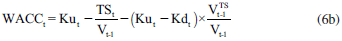
This formulation assumes that the market cost of debt is identical to the contractual non-capitalized cost of debt.
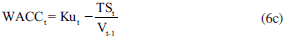
Assuming ψ = Ku:
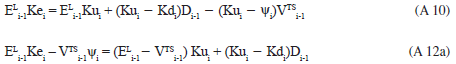
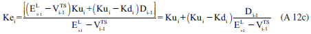
Assuming ψ = Ke:
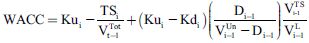
See Kolari and Vélez-Pareja (2012) and Appendix for a derivation.
Where VUn is the firm unlevered value; other variables already defined.
Examining the formulas for the WACC tax savings might be included explicitly in its formulation. This has the advantage that all types of tax savings can be introduced in the analysis, as suggested in Section Two.
CONCLUDING REMARKS
This paper presents a step-wise function for the calculation of TS with and without losses carried forward and with financial income and explains how to use it in a correct the WACC formulation. In addition, it demonstrates that the condition for a firm to earn TS is not that it pay taxes but that it should be subject to taxes and that the EBITAdj should be positive. This step-wise function applies to all cases regarding the relationship between EBITAdj and FE.
It is therefore apparent that the traditional textbook formula cannot be taken as the standard. Using the formula in all cases may result in the overestimation of the valuation of cash flows, see Kaplan & Ruback (1995), because disregarding the real role of TS leads to the underestimation of the WACC. A general formulation from Taggart (1991) and Tham and Vélez-Pareja (2002, 2004) was adopted, whose TS and the values for the TS are explicitly included in the calculation of the WACC. This approach opens up possibilities for considering sources of tax benefits that are not directly related to the interest that firms pay.
As was shown above, when a firm's OI includes interest income, differences between the tax liability in unlevered and levered firms are not identical to TS. Adjustments that take into account the difference between financial OI in levered and unlevered firms are required when this situation arises.
A future line of research would be to measure the size of TS for the traditional approach and compare it with the procedure proposed here. In point of fact, the author is currently supervising final-year graduate MBA research on this topic. A student is conducting an estimation of the over- and undervaluation of the size of TScalculated using the traditional textbook value and the approach proposed in this paper. The results of this research will be a matter for a future paper. The firms to be analyzed are taken from the S&P Capital IQ Database. The student has collected information for more than 2,100 firms, for a total of 21,769 observations after "cleaning" the database and selecting the appropriate observations required for analyzing the TS.
A drawback is that, in cases where LCF are allowed, calculating TS poses a problem of "counting down" the TS lost in previous years but that might be recovered in the future. This drawback is easily solved, however, either by using a good spreadsheet program or by valuing the firm using the Capital Cash Flow technique proposed by Ruback (2002) and assuming that the discount rate of TS is Ku, the cost of unlevered equity. In this last case the discount rate (shown in the Appendix) is free from the calculation of TS: it is simply Ku, the cost of unlevered equity.
This article provides practitioners with a simple and correct procedure to calculate the amount of TS a firm is able to earn, which they are able to use in order to arrive at a better estimation of the WACC. This paper invites researchers and practitioners to abandon the practice of using the standard textbook formulation of the WACC and to incorporate explicitly estimated TS in their formulations of the cost of capital.