English (pdf)
 Article in xml format
 Article references
 Send this article by e-mail
 Cited by SciELO
  Cited by Google
  Similars in
SciELO
Similars in
SciELO  Similars in Google
 Permalink
INTRODUCTION1
Fertility trends among the poor, measured as the average number of children per woman, have been decreasing in most developing countries during the last years with the exception of Africa. It seems that the current problem is not only about the number of children poor women bear, but the age at which they have their first child. Table 1 shows a representative sample of 41.344 Colombian women aged 20 to 49. The second and third columns correspond to the percentage of women who have given birth before the age of 18 and 23, respectively. Given its high incidence in all income level groups and especially among the poor, early childbearing is the issue of interest here. The third column of Table 1 shows that poor Colombian women have, on average, twice the number of children compared to wealthy women, which may also be related to their early entrance into motherhood.
Table 1 Age at First Birth and Average Number of Children
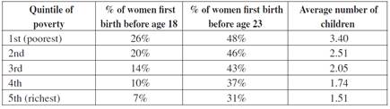
Source: Calculations from DHS - Demographic and Health Survey, Profamilia (2005).
Is there any value in a young woman postponing childbearing? This is the main question that this paper seeks to answer. The existing literature concerning the relationship between early childbearing and future socioeconomic attainments of young mothers shows us very divergent conclusions. A group of studies concludes that early childbearing considerably affects the future performance of women, constituting a negative event without which the young mother could reach higher attainments. Another group of studies assures that the poor performance of some young mothers is not the consequence of their early entrance into motherhood. Instead, their disadvantaged background prevents them from doing better regard-less of the presence of a child. The existing divergency in the current literature on this topic makes our research question worthwhile.
Classifying studies according to the methodology employed, there are four identified groups: i) those treating age at first birth as an exogenous variable affecting certain socioeconomic outcomes of the mother, e.g. Waite and Moore (1978) and Williams (1996). These studies find considerable negative effects of early motherhood on women’s achievements. ii) Papers using Instrumental Variable techniques, e.g. Klepinger et al. (1999a, 1999b). Early entrance into motherhood is treated as an endogenous variable. This group of studies finds a lower -compared to i)- but still important negative effect on future performance of young mothers. iii) Studies considering a control group - e.g. sibling comparisons (Geronimus & Korenman, 1992; 1993), classmates matching (Levine & Painter, 2003). IV) those derived from a natural experiment -e.g. twins comparisons (Grogger & Bronars, 1993), teen mothers experiencing miscarriages (Hotz et al., 1997). The two latter groups of studies find only a small effect of early childbearing on women’s future socioeconomic attainments, concluding that preventing childbearing does not guarantee a considerable increase in achievements of already disadvantaged mothers. Those results cast doubts on the direction of causality from early child-bearing to low socioeconomic achievements that was assumed in the earlier contributions on the topic. In fact, not taking endogeneity into account seems to be a considerable source of error.
What is, therefore, the right direction of the causality in the relationship between early childbearing and schooling attainments or any other socioeconomic achievement? The argument based on the evident time rivalry between being a mother and studying, may be used to support either causality direction: On the one hand, early parenthood may prevent young mothers from spend time in schooling investment, and, on the other, given the time rivalry between the two activities (motherhood and human capital accumulation), women with high schooling expectations prefer to postpone childbearing. Indeed, there is a general acceptance of this last idea (Rindfuss et al., 1984). In addition, previous studies have questioned the direction from young motherhood to low educational achievements. We have already mentioned the conclusions of the group of studies using natural experiments to check the causal effect of teenage childbearing on a teen mother’s subsequent socioeconomic performance: preventing early childbearing does not ensure an improvement in achievements of already disadvantaged mothers. Another contribution in this direction is the paper by Upchurch and McCarthy (1990). They find that adolescent maternity does not always lead to educational deprivation; controlling for social background and personal features, childbearing does not increase the probability of leaving school. Haggstrom et al. (1981) find no support for the negative effects of teenage parenthood on ambitions and attainments. Although it is true that non teenage parents perform better on most of the measured outcomes -educational, vocational, and personal development- than their classmates who experienced an early entrance to parenthood, the differences are explained by other characteristics pertaining to the individuals and their environment rather than early childbearing. In addition, Kantorová (2002) find that highly educated women postpone childbearing even beyond the end of schooling, because they want to form their position in the labor market before their entry into motherhood. On the contrary, women with no universitary degree have restricted prospects on the labor market. Thus, they are less motivated than more educated women to postpone childbearing in order to construct their labor career.
Finally, another stream of the literature worth mentioning here is the one related to survival models, where the determinants of birth spacing are explored by estimating hazard ratios. Those studies analyse, among other issues, the role of education in driving childbearing postponement, finding that schooling actually contributes to delay entrance to motherhood (See for instance Gangadharan & Maitra, 2003; Tavares, 2010).
There might still be controversy on this issue, but it is definitely very plausible that having high schooling goals causes delay of the first childbearing experience2. This is the direction of causality we are exploring here, giving great importance to the costs of early maternity in terms of future educational achievements. It can-not be denied that there are other cost of childbearing such as forgone wages, job opportunities, giving up the consumption of some private goods, travel opportunities, social networking, among others. However, in this paper, we have chosen to analyse a reduced form of the cost; i.e., the forgone schooling investment. We do this because such childbearing costs evolve with time as suggested by the model used here.
We will use a real option model (Dixit & Pindyck, 1994) to explain under which circumstances a young woman would be better off delaying her first childbirth experience. A firm must take into account future costs and opportunities when deciding whether or not to invest. Likewise, a woman should consider the same factors when deciding the optimal time to have her first child, given the irreversibility of her action. As far as we know, Iyer and Velu (2006) were the first to use the real option approach to model the timing of the women’s decision to have children. In their model, the net benefits of children are subject to uncertainty, which determines the ‘value of waiting’ and, therefore, the spacing and delay of an additional child. The added value of this paper compared to I&V and other previous contributions is that we further explore the costs of an early first childbearing, emphasising the way those costs evolve in time. Additional contributions are the analysis of the decision making process according to the socioeconomic background of women and the calibration of the model based on Colombian data.
We use a real option approach because it seems to be suitable to model the rational choice of a woman deciding the age she wants to enter into motherhood, since the costs she faces by exercising the option of having the first child are decreasing and uncertain. The approach is useful to give theoretical support to the argument that high educational aspirations lead to rationally postponing childbearing.
In our model, a woman chooses the optimal age to have her first child; i.e., the age at which the net benefits of childbearing are maximised. A relevant point is that a simple Net Present Value (NPV) evaluation is not enough to carry out the right decision. There might exist a positive ‘value of waiting’ that should be considered as well. Early childbearing is an appropriate case to analyse in the context of option value theory, since first, its costs are at least partly irreversible (unrecoverable sunk costs), and second, the decision can be delayed so that the woman has the opportunity to wait for new information to arrive about uncertain costs. It is worth adding that the NPV and ROA approaches would potentially coincide in the case without uncertainty (but decreasing costs). In fact, the main argument exposed by Dixit and Pyndick (1994) for using ROA instead of NPV is that, under uncertainty, the critical value of the investment that makes the decision optimal is greater than the one given by the NPV rule.
In many cases, bearing a child as an adolescent is more by accident than by choice3. However, this unplanned event is the result of a sequence of decisions or choices the woman has made before. The first choice is to have sexual intercourse; the second is to do so without using contraceptive methods. If pregnancy occurs, a woman may choose to interrupt it, either legally where this is possible, or illegally as often occurs in countries with prohibitive abortion laws. Following this reasoning, even when early childbearing has been an accident and not a choice, it is an unplanned consequence of a sequence of previous choices.
Clearly, we are assuming that first childbearing is an individual choice. However, this might be, in many cases, a family choice. We do not deny this point but con-sider that our way of modelling is still appropriate: each member of the couple, before making a family decision, has to make his/her own decision. It is precisely this individual decision that we analyse here.
Section 2 presents the model. Nature has given women an investment opportunity, namely, the possibility of bearing a child at any time from menarche to menopause. This investment opportunity, as any other investment, carries both benefits and costs. To decide on a conventional investment project, it is enough to ponder benefits and costs in order to determine the optimal time to invest. This is not the case of the investment opportunity we are analysing here, since the costs of bearing exhibit both uncertainty and decreasing behaviour through time. This generates a value of postponing that a woman should consider if she wants to optimally decide the timing of her first child. From the maximisation problem, the critical value of the cost of childbearing is obtained. This critical value or threshold deter-mines when it is worthwhile or not for a woman to delay the time she has her first child. The optimal age corresponds to the time where the cost of bearing equals the critical cost.
In Section 3, the implications of differences in women’s socioeconomic background are analysed. In Section, 4 we calibrate the model using Colombian data corresponding to fertility and socioeconomic characteristics of women. We analyse three types of women according to their poverty level. Using real data, the initial cost of bearing and its evolution in time is calculated. In Section 5, some comparative statics are carried out in order to simulate changes for the relevant parameters. The exercise illustrates the main implication of our analysis: if opportunities to reach high educational achievements were not dependent of a woman’s socioeconomic background, she would rationally choose to have her child at an older age. In other words, early childbearing by impoverished women might be seen as a rational reaction to their disadvantaged situation, where opportunities to reach high achievements are low, regardless of the presence of a child. Before concluding, in Section 6, we briefly discuss some relevant topics related to the timing of the entrance into motherhood; i.e., the number of desired children, the option of abortion, and the implication of differences in women’s abilities. Finally, Section 7 presents the conclusions.
THE MODEL
We consider the act of bearing the first child as an investment decision for the woman. Women are rational agents who consider the information at hand to optimally decide the age at which they have the first child. As with any investment, bearing a child brings benefits and costs. The benefits include, for instance, happiness and support in old age. The costs of childbearing can be thought of as opportunity costs, since there is rivalry between the time and income that a woman could assign to many other activities including investment in education (which affects future wages), social networking, traveling, and work experience, among others.
At each year t = 0, 1,...T, from the age of menarche (t = 0) to the year before menopause (t = T), women have the option to either bear a child and forego the potential benefit of waiting, or postpone the net benefits of motherhood and keep the value of waiting to invest (see below for a definition of the value of waiting). This is analogous to holding an option in the financial market: at any time t, a woman has the right but not the obligation to bear a child at a given cost. In this sense, a question that we are interested in answering is: what is the rule that maximizes the value of the investment opportunity that a woman holds? Let us not forget that the decision of having the first child is irreversible, while waiting is not (at least up to T).
Let us denote the option value or the opportunity of investment that nature has given to women as F (C), which represents the objective function that they aim to maximize. Writing the payoff from having a child at age t as the difference between the benefits and the costs B − C t , the goal will be to maximize its expected present value-

Where p is the discount rate, which has the usual interpretation: how women value the future with respect to the present. Here we are assuming that the benefits of children - happiness, support in old age - are constant. This is done for the sake of simplicity, as our main concern is the nature of the evolution of the costs in time. Still, we can give at least two arguments to justify benefits being constant4; first, given that support in old age is expected independently of the timing of birth, this type of benefit can be regarded as constant. Second, existing literature suggests that happiness brought by children will be the same regardless of the age of first childbearing. For instance, Myrskylä and Margolis (2014) find a very small effect of children on happiness after the first year; even for those studies finding a longer-lasting effect, e.g., Baetschmann et al. (2016), results show that these effects vanish after (around) ten years. It seems then plausible to consider B as constant.
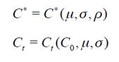
The maximisation process where a woman chooses t to maximize will lead us to obtain a critical value of the cost C ∗ or threshold, C t having the first child.
How do the costs of childbearing evolve in time? It is proposed here that the costs of bearing are subject to uncertainty and that they decrease over time. They can be formally represented by a mathematical expression that captures both characteristics: the stochasticity of the variable and the negative drift; a good candidate for this purpose is a geometric Brownian motion, which is commonly used in Finance to analyse entrepreneurs’ investment decisions where net benefits are not certain and are irreversible (in the same way as childbearing is). Thus, C t may be represented as follows5.

where p>o is the instantaneous conditional expected change in costs per unit of time, is the instantaneous conditional standard deviation per unit of time, and dz is an increment to a Wiener process6.

With  Both the potential decrease in the costs of childbearing and the uncertainty create a value of waiting. Indeed, it is important to note that even in the deterministic case; i.e., when there is no uncertainty in the costs (σ=0), there might still be a value in waiting.
How to explain the negative drift or decreasing trend? One of the reasons for the childbearing costs to decrease in time (negative sign next to µ) is the reduction in the forgone educational investment in time: as a woman gets older, she either has already progressed a long way in the construction of her human capital, or the chances for her to begin the construction are very low. Thus, the younger a woman is, the higher her cost in terms of forgone schooling investment. The same ration-ale may be used for explaining the decreasing cost in terms of future highly paid jobs, since human capital is a major determinant of earnings. The opportunity costs in terms of forming a position on the labor market also decreases in time. This is because, as a woman gets older, her opportunities to start constructing a labor career shrink. The younger a woman is, the more time she has to grow professionally. In the calibration section, the decreasing tendency of educational costs is illustrated, using real data from Colombia.
As for the uncertainty of childbearing costs, one may identify several sources. Let us focus on the educational costs. A woman may fail in predicting i) if her parents or she will be able to financially support her future studies in the presence of a child, ii) if her ability7 is high enough to continue in higher education, iii) whether there will be an availability of credits or scholarships for her to continue studying (incomplete capital markets), iv) or available job market opportunities. The opportunity costs of childbearing may go up or down depending on these conditions that are not certain. Thinking of the costs in terms of labor market prospects, there is also uncertainty in how costly it would be for a woman to give up a period of life that she could spend in achieving a position in the labor market. The uncertainty would be higher or lower depending on several factors such as her socioeconomic background, and social networking, among others.
Solving the Maximisation Problem
We will now show the way to solve the basic problem by using dynamic programming. We are dealing here with what is known as a stopping problem, where stopping corresponds to bearing the first child and continuation corresponds to postponing childbearing. While a woman holds the option (while she waits and does not bear), the only pay-off that she receives is the change in the value of the investment opportunity F8. Hence, the Bellman equation for this problem is obtained by equalising the expected return of the investment opportunity with the expected change in the value of the investment opportunity,
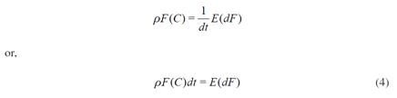
Equation (4) says that a woman’s decision is optimal only if the benefit from holding the option equals the cost of holding it (forgone benefit of exercising the option). This Bellman equation applies for values of C higher than the critical cost -where it is worthwhile postponing childbearing-. The critical cost is the threshold that will be obtained by solving the optimisation problem9. Using Ito’s lemma to expand dF, we obtain:

substituting in, and substituting dF in (4), we obtain the following second order differential equation:

where we have used E ( dz) = 0, E ( dt)2 = 0 and E(ε)2 = 1. Equation is a second order differential equation with the standard general solution given by a linear combination of two independent solutions.
In order to obtain C∗ and F, we should impose three boundary conditions on F (C). The first condition states that:
which means that the investment opportunity F is of no value when the costs of childbearing tend to infinity10.
A second constraint is the so-called value matching condition, according to which the investment opportunity F equals the net benefit B − C at the critical value of the cost (C∗)
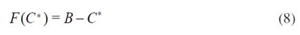
This condition simply means that, once childbearing occurs, the woman obtains the net benefit as a pay-off11. The objective function will be maximised only if the option of bearing is exercised at the optimal time, i.e., when there is no value of waiting.
Finally, the smooth pasting condition requires to hold when taking derivatives at both sides of the equation with respect to C (at C∗).
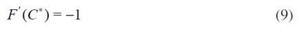
The smooth pasting condition requires that, for the threshold cost level to be optimal, a small change in C∗ will have no first order effect on the net gain from bearing a child, where the net gain is defined as follows: if the woman decides to postpone bearing, she keeps the investment opportunity F (C). If she decides to bear a child, she obtains B - C but loses F (C). This difference ( B − C − F (C) ) constitutes the net gain. The optimal choice of C∗ implies the smooth pasting condition (Hogan & Walker, 2005).
We start the solution of this optimisation problem -to solve subject to the three boundary conditions- by guessing a solution for F ,

Hence,
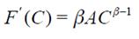
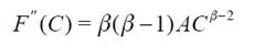
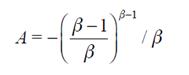
Where A is a constant to be determined and β is a root of the following characteristic equation,
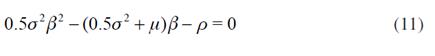
which we have obtained by replacing F, F' and F'' in. The roots of are given by:
Where β1 > 0 and β2 <0. The general solution can be expressed as:
However, for boundary condition to hold, A1 should be equal to zero and the expression reduces to 12. We use the value matching condition and the smooth pasting condition to obtain C∗.
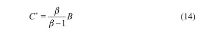
The fraction on the RHS of is positive and lower than 1, which implies that, in the optimum, the benefits of bearing a child must be higher than the critical value of the costs. The size of the wedge  depends on the values of σ and µ: the higher the parameters, the closer the wedge is to zero and the higher the difference between C
∗ and B at the optimum. We further analyse this point in the next section.
depends on the values of σ and µ: the higher the parameters, the closer the wedge is to zero and the higher the difference between C
∗ and B at the optimum. We further analyse this point in the next section.
Optimal childbearing decision-making path
Figure 1 shows the optimal childbearing decision-making path. In panel (a) we see both, the F curve and the NPV curve, where the three boundary conditions are satisfied: 1) F goes to zero as the cost tends to infinity, 2) at the critical point the woman gets B − C ∗ as a payoff, and 3) at the optimal level, the two curves are tangent, which is precisely the meaning of condition. This is because the value of the investment can never be lower than B − C.
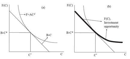
We replicate the graph in panel (b) in order to highlight the investment opportunity function, which corresponds to the bold line. Wherever C > C ∗, it is always better for a woman to wait, since the curve F lies above the net benefit line B − C. This is true until C = C ∗, where there is no value in waiting and the woman exercises her option to have a baby, getting the payoff B − C ∗.
It is less straightforward to explain why the value of waiting is zero when C < C ∗, given that the curve F is again above B − C. The reason is that for values of C lower than C ∗, the difference between the curve F and B − C can no longer be interpreted as the waiting value: this value would always be high because the out-look of facing lower costs would imply an even higher value of waiting for a child that will never come13. Dixit (1992) called this phenomenon a “speculative bubble”, for the case of an investment project subject to stochastic benefits. Therefore, when C < C ∗, the optimal path is simply given by the net benefit line B − C and not by the curve F.
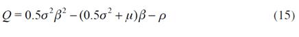
Equation tells us that C* depends on the strength of the decreasing trend, the uncertainty and the discount rate. In fact, β increases with σ and µ; i.e., the more uncertainty about future cost and the higher the decreasing tendency of these costs in time, the higher the value of postponing childbearing (Equation implies that ∂C*/∂β<0). We can easily verify this as follows. Let us first define the characteristic equation as Q,
Totally differentiating Q with respect to σ and then µ, we have,
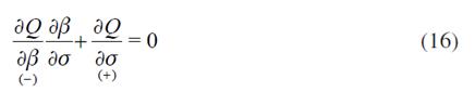
where  , and
, and  . Hence,
  for (16) to be true. Likewise,
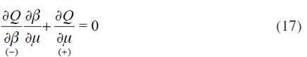
where , and  . Hence
  for (17) to be true.
The discount rate p is also relevant in determining the position of the critical value of C*. Totally differentiating Q with respect to, p
where  . Hence,
  for (18) to be true.
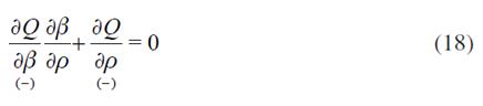
To better illustrate the impact of the parameters, let us compare the equilibrium situation of two different women, one experiencing a higher level of uncertainty than the other. Ceteris paribus, a higher implies a change in the slope of the F (C) curve (counter-clockwise rotation) and, therefore, a shift to the left of the critical cost C
∗. As we can see in Figure 2, the investment opportunity curve that represents higher uncertainty, is above the other curve. This means that women with higher uncertainty obtain greater value from waiting. For them, the critical cost level is lower, and the expression  is closer to zero; thus, the difference between the benefits and the costs at the optimum level is higher.
A similar analysis applies for Ceteris paribus, a higher implies a flatter F (C) curve and a lower value of the critical cost C ∗. This means that women with a higher decreasing trend of the cost obtain a greater value from waiting. As for women with higher discount rate, ceteris paribus, will have a lower value of waiting.
It is relevant to notice that the optimal age for first childbearing, at which C t = C ∗, depends significantly on the initial cost or the cost at the age of menarche for each woman. The higher the initial cost, the higher the value of waiting.
DIFFERENCES BETWEEN TYPES OF WOMEN
In this section, differences in women’s socioeconomic background are taken into account. Here we use the example of poverty groups, although the same exercise could be carried out for ability with no major variations. We briefly consider the implications of differences in ability in Section 6. The focus will be on educational costs of childbearing but, again, other kinds of costs could be analysed for different groups of women, probably with some variations in the conclusions.
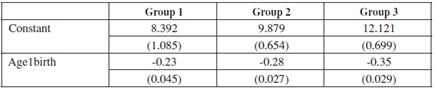
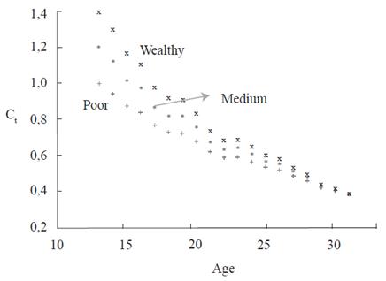
Let us define three types of women: Type 1 - poor, Type 2 - medium income, Type 3 - wealthy. Women from all groups behave rationally and consider the same factors when deciding the optimal age t ∗ for their first childbirth. According to the real option model analysed here, the initial cost C 0, σ , µ and p are the relevant parameters determining the optimal decision. How can we expect the values of these parameters to differ among types of women, which makes the optimal age be different as well?
Starting with C 0, let us compare women from each of the three types at the age of menarche. The potential achievements in terms of schooling, high wage future jobs, travels possibilities, for instance, are the lowest for the poorest type. They would potentially give up less than their wealthier counterparts if an event such as childbirth occurs. This reasoning certainly applies to developing countries, where the opportunities to reach high educational levels and the chances for high wages jobs are much lower for the poor, and poverty affects around half of the population. Then, we have that C 1 0 < C 2 0 < C 3 0 . The value of waiting or delaying childbirth would be higher for the wealthier type.
As for p , there is evidence in the literature suggesting that people from lower socioeconomic backgrounds have higher discount rates than those from higher socioeconomic background (See for instance Harrison et al., 2002). We would expect then that p1 > p2 > p3. Having a high discount rate reduces the value of waiting, thus, poorer women will be less willing to delay their entrance to motherhood.
Focusing now on σ, it is reasonable to expect that this might be lower for Type 1 women. The intuition is that for poorer women, the chances of reaching high socioeconomic achievements, including high education levels, are low regardless of the presence of a child; i.e., they experience the lowest uncertainty. In the same line of reasoning, uncertainty on childbearing costs would mainly affect the middle income group: women in this group are assuming a higher risk, since their income might not be enough to bear both childbearing costs and educational costs. As for the wealthier population, given that their income might be sufficient for both child and school, one could expect their uncertainty level to be lower than for the middle group. Still, compared to the poorer population, their uncertainty level should be higher, since there is still rivalry between the time spent in childcare and schooling investment, which for them is potentially high.  1 <
1 <  2 , 1 < 3 , and possibly 3 < 214.
With respect to  let’s recall that it represents a decrease in time in terms of the cost of childbearing, namely forgone educational investment, labor market opportunities, or any other opportunity cost. Thinking of educational costs, as it has been mentioned, women with high incomes have a higher level of potential educational achievement than low income women. Thus, their opportunity cost of bearing is higher, the further they are from reaching their potential educational level (the younger the mother is). However, as time goes on, once the opportunities to invest in education decrease for both high and low income women, the costs of bearing for the two groups tend to zero, given that educational achievements are most likely to be realised within a given time window. This means that those women who begin with a higher initial cost, experience a higher decreasing trend of their cost 1 < 2 < 3.
One may instead argue that richer women have a greater time frame for the cost of bearing to converge to zero, since their educational aspirations are, from the beginning, higher. However, there is a factor making it reasonable to use a similar time window for the three types: impoverished women are more likely to experience periods of school desertion. Eventually, they would have to drop out of school, join the labor market or stay idle, and go back to school some time later. This stretches their time window and makes it comparable to that of wealthier women. However, this may not be the case if other kinds of childbearing costs different to forgone education were analysed; for instance, the costs in terms of forgone wages. In that case, the time window for richer women would be potentially higher.
In the calibration section, convergence has not been imposed, but the data reveals it. There, the cost is defined as the difference between the potential schooling level and the observed average schooling at each age of first birth. It is observed that the costs for the three types converge to zero at a more or less similar time window, since older mothers are closer to the potential schooling achievement of each type.
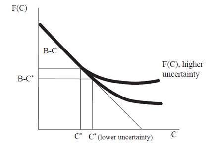
Figure 3 illustrates how the optimal path would hypothetically differ between the three types of women. The critical value of the cost C∗ for Type 1 women is closer to 1 because of their lower µ and σ, and their higher discount rate. Likewise, the optimal timing for first bearing, at which Ct = C∗, is at a younger age for Type 1 women because of their lower initial cost. This hypothesis about the difference in the optimal age between types, t1∗ < t2∗ < t3∗, will be dealt with in the calibration in Section 4.
CALIBRATION
In order to illustrate the women’s behaviour described above, in this section, we will replicate the model using Colombian data. The database comes from the “National Survey of Demography and Health” (Profamilia - Colombia) and was carried out in 200515 and includes a representative sample of 41.344 women aged between 13 and 49.
In short, we have the following for the critical cost and the cost of childbearing at any time t,
Where C0 is the initial cost. As it was announced earlier, the focus is on the educational cost of childbearing. We divide the population into three types: poor, medium and wealthy. The potential problem of this division is that it takes into account the current socioeconomic situation of the woman, as the survey does not tell us about her background at the age when she has her first child. However, this is not really problematic if we consider that empirical evidence has shown that Colombia is a country with very low social mobility (see for instance Gaviria (2002) and Andersen (2001)). This means that the socioeconomic ranking of women from poorer to wealthier is not expected to have changed significantly.
The cohort chosen for the analysis comprises women aged between 25 and 35 (11.879 women). The selection of this cohort attempts to consider two factors: first, there is a potential truncation problem if young mothers enroll for formal education later. Although it is not possible to know with certainty how many of those women in our sample will not attend the educational system anymore, we can check the current situation. According to the Profamilia survey, the oldest women currently attending a formal educational institution are 24 years old. Second, including older women in the analysed cohort would ignore the fact that in the past, education coverage was lower. Thus, we could not attribute the lower observed schooling to an early childbearing. Women of this age range were all supposed to have begun school during the mid-seventies and after. From this decade onwards, the coverage rates of education have increased significantly in Colombia for all social levels. This makes the sample more easily comparable.
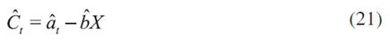
Let us start by obtaining Ct for the three types. The observed cost at any point in time is defined here as the difference between the potential schooling for each type ( Sp ) and the observed average schooling of women having their first child at each age ( St ),

which, as expected, decreases in time. Sp corresponds to the mode of schooling years among non-early mothers, namely, those that have their child when they are older than 23 (8.4, 12.5, and 16 for types 1 to 3 respectively). In order to obtain values µ of σ and associated to the database, we use the following result for a geometric Brownian motion; i.e.,

are N ~ (µ, s2) variables. Although Ct , as defined in , presents a decreasing trend, the log is undefined in some cases when the value inside the parenthesis is negative, which happens when the observed schooling is above the potential. To avoid this, it is needed to smooth the relationship between Ct and the mother’s age when she gives birth for the first time ( X ), by regressing Ct on X16. The estimated coefficients ( and b ) are used to calculate:
The previous procedure allows us to obtain, from (20), the following values for and by types:  ,
,  ,
,  ,
,  ,
,  ,
,  17.We see that

 and
and 
 . This is consistent with the intuition presented earlier in Section
  , except for the of the middle group, which was not the highest as expected. Normalising the initial cost (the cost at the age of menarche), we obtain
  ,
,  and
and  (these are the relative initial costs of each type with respect to ).
Considering the Brownian motion, we have the following:
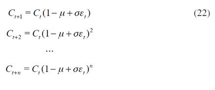
Figure 4 shows how these costs tend to converge for all types at the end of the analysed period, reflecting the assumption discussed earlier, namely that the forgone educational investment decreases in time. It is also observed that the initial cost is the lowest for the poorest type. The curves in this figure have been obtained by applying the evolution of the costs described in to each C0.
Source: Authors based on DHS - Demographic and Health Survey, Profamilia (2005)
Figure 4 Evolution of the Cost of Childbearing in Time
In order to estimate the optimal age of childbearing for each type, we would have to know the value of t at which Ct = C ∗. Likewise, for calculating the critical value of the cost, we would have to know the value of the discount rate for each type, which is unknown and cannot be calculated using the real data. One possibility to continue the exercise is to choose the current situation as a benchmark. This is, to assume that Colombian women behave optimally according to the model analysed here. Thus, the observed average age of first childbearing for each type is taken to be the optimal age (20, 23, and 25 for each type respectively).
The critical costs are  ,
,  and
and  . Although these values are close to each other, let’s recall that the initial cost is lower for the poorest than for the wealthiest, which implies that the continuation region is shorter for the poorest, as mentioned above. Using this numbers and normalising the benefits of childbearing to
  18, the discount rates that make the critical value equal to
  at each optimal age are
  ,
,  , and
, and  . Although the difference is not very big,
  is indeed higher than
  , as the existing literature on discount rates' differences by socioeconomic background suggests.
The next step is to calculate both the value of the investment opportunity  at each time - given by
  - and the net present value
  at each age, in order to visualize the optimal childbearing path for each type of woman, where
  as it is expressed in Equation (12).
Solving for  in (13) and replacing
  from (14) we obtain,
Thus, the investment opportunity F for each type is as in Table 2 (using (10)).
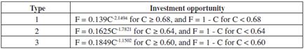
Now, it is possible to illustrate the optimal timing of first childbearing and the optimal childbearing decision path. Figure 5 plots both the NPV curve and the F curve as a function of the age of first bearing for the three types of women. At the critical point, the NPV curve is tangent to the F curve (smooth pasting condition).
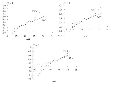
Source: Authors based on DHS - Demographic and Health Survey, Profamilia (2005)
Figure 5 Optimal Timing of First Childbearing and Investment Opportunity
We can also illustrate the values of the investment opportunity F as a function of the costs. This is done in Figure 6. We observe that the critical value of the cost (tangency point of the NPV and F curves) is further from the initial cost as we move from Type 1 to Type 3 women. The continuation region (where it is better to postpone bearing) is shorter for the poorest type.
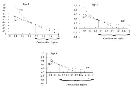
Source: Authors based on DHS - Demographic and Health Survey, Profamilia (2005)
Figure 6 Investment Opportunity and Critical Point
SIMULATION
Let us now simulate changes in C o and the relevant parameters for Type 1 women -the poorest group-.
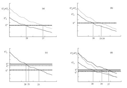
Figure 7, panels ( a) and (b) show the increase of the optimal age for first bearing if, ceteris paribus, the initial cost of the poorest group is set as equal to the initial cost of the other two types ( C 1 0 = C 3 0 and C 1 0 = C 2 0 respectively). If the initial cost of Type 1 women were as high as the cost of the wealthiest group, the optimal age would increase to 27 (the age at which C 1 ∗ = 0.68 ). For the second case, the optimal age changes to 23-24 years.
Source: Authors based on DHS - Demographic and Health Survey, Profamilia (2005)
Figure 7 Simulations for the Poorer Group of Women
Panel  shows the impact of a change in poor women’s preferences with respect to the discount rate
  .
.  corresponds to the critical cost if
  , where the optimal age increases to 21 years. If the discount rate halves,
  , the optimal age increases to
  years, with a critical cost
  .
.
Finally, panel  shows that the optimal age changes to
  if, keeping the same discount rate preferences,
  ,
,  and
and  are set as equal to those of Type
  .
.
It is important to emphasize the relevance of the initial cost in determining the value of waiting. This suggests that, as long as the possibilities of poorer women to reach high educational achievements increase, they will optimally choose an older age to begin childbearing. Thus, it is suggested that an antipoverty policy consisting of increasing the possibilities of poorer women to reach higher levels of education in spite of their income constraints, may be more effective than fertility policies to prevent childbearing: a higher expected (educational) cost would rationally motivate women to postpone childbearing. If the educational policy is successful, and the opportunity to reach high educational achievements does not depend of one’s socioeconomic background as it does currently, this would work as a transformation from Type 1 to Type 3 (at least in terms of the parameters values).
BEFORE CONCLUDING
Before concluding this paper, it is interesting to briefly take into account three relevant features that have not been considered in the previous analysis and that are related to the timing of first bearing. First, the number of children that a woman wants to have, which may influence the timing of entering into motherhood. Second, the heterogeneity in ability among women, which implies different potential costs of early childbearing and may determine differential incentives for postponing the first bearing. Finally, some stylised facts regarding the choice of abortion.
Number of children
So far, we have not mentioned a relevant aspect that may also affect the timing of the first birth: the number of children desired. The more children a woman wants to give birth to, the earlier she would -most probably- begin bearing. In the Profamilia survey, mothers and women who are not yet mothers are asked the exact Number of children they would like to or would have liked to have19. Table 3 shows the percentage of women according to the desired number of children, for early and late mothers (women 25-35 years old).
Table 3 Percentage of Women by Number of Desired Children
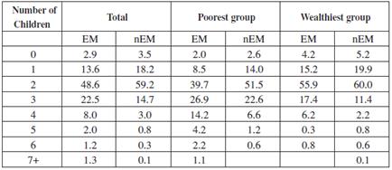
EM: mother before 23 years old. nEM: mother after 22 years old.
Source: Authors based on Profamilia - Colombia
First, it is observed that early mothers want to have more children than late mothers: while 35% of early mothers want to have 3 or more children, only 19% of late mothers would like to do the same. Second, early mothers of both socioeconomic groups -poor and wealthy- want to have more children than their late mother peers, 48.6% (24.7%) and 31% (15.1%) of poor (wealthy) women want to have more than 3 children. And third, wealthier women, both early and late mothers, want to have fewer children than poorer women. This is consistent with the existing literature relating income with quantity of desired children and does not contradict what we have been analysing in this paper. Poorer women have a lower opportunity cost of bearing a child, which influences both the quantity of children they would like to have and the timing of their first birth.
Differences in ability
The opportunity cost of childbearing may vary according to the ability of the woman as well. A potential mother with higher ability faces higher potential costs in terms of forgone schooling investment and forgone highly-paid job positions.
this is a component of heterogeneity among women that is not considered in the paper and plays a potentially important role in the timing of first bearing. We can attempt to introduce ability into the analysis in two ways. First, as mentioned in Section 3 for different socioeconomic groups, we may identify three types of women according to their ability low (1), medium (2), and high ability (3). The initial cost for each type would be ranked as C 1 0 < C 2 0 < C 3 0 . The value of waiting or delaying childbirth is higher for the type with the highest ability level. Low ability type women would have little chance of obtaining high educational or labor achievements, regardless of the presence of a child, while the high ability women would rationally delay childbearing.
Second, we could analyse heterogeneity in ability within each socioeconomic group. A poor woman with high ability, as long as she can access (good quality) public education or scholarships, can potentially achieve high future outcomes. Her initial costs of bearing would be higher than her peers and she would ration-ally choose to postpone bearing. An analogous analysis applies for wealthy low ability woman.
The choice of abortion
An early pregnancy does not necessarily end in early childbearing. A woman can choose to interrupt her pregnancy, or a miscarriage or a health problem may occur. If abortion would be legal everywhere and no ethical, moral and religious aspects were influential in a womans choice to terminate her pregnancy, one would expect, according to the model analysed here, that poor (or low ability) women would have less incentives to delay bearing or interrupt a pregnancy. Table 4 shows some statistics from Colombia. Because abortion is illegal in this country, cases of deliberated termination of pregnancy are expected to be underreported.
Table 4 Percentage of Women that Interrupt Pregnancy
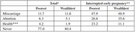
* Women from 25 to 35 years old
** Women (25-35 years old) who experienced an interrupted pregnancy before the age of 23.
*** Extrauterine pregnancy or fetal death
Source: Authors based on Profamilia - Colombia
The two last columns of Table 4 show that, among those women that have interrupted pregnancy at an early age, a higher percentage of wealthier women, compared to the poorest group, have chosen to have abortions. This is expected because wealthy women have more incentives to delay childbearing than poor women, an important feature analysed in this paper.
We would also expect for poor women to be more exposed than wealthy women to interrupted pregnancies. The second and third columns of Table 4 confirm this, although the difference between the two groups is not high. The features that most influence the difference are the interrupted pregnancies due to extrauterine pregnancy or fetal death, which are more common among the poorest group.
CONCLUSIONS
This paper deals with the problem of early childbearing. Although this phenomenon affects all social classes in all countries, young motherhood is still experienced most frequently among the poorest women. We have used option value theory to analyse under which circumstances it is worthwhile for a woman to post-pone her first birth.
The (educational) costs of bearing tend to decrease in time and they are subject to uncertainty. Both factors create a value of waiting, until a critical cost or threshold is reached. The analysis is made for different types of women, according to their socioeconomic or personal characteristics. We highlight the fact that middle and upper income women face higher initial costs of bearing, higher decreasing rate of the costs and higher uncertainty. This increases the value of waiting for these women more than for the poorest women.
An important issue involves the policy implications for the poorest groups of women. The message of the paper is that policy measures aimed at reducing early childbearing are helpful since even this type of women obtain a positive value from waiting. However, as antipoverty policies, policies for the prevention of early motherhood are very limited: poor women’s relatively lower achievements will still exist regardless of whether they have children or not. This is why we used a lower initial cost of childbearing in our simulations. The fact that poor women face lower uncertainty in terms of the cost of childbearing, in the sense that they very likely will perform poorly with or without a child, reduces the value of postponing.
The previous reasoning suggests that educational policies to allow poor women to access the schooling system have an additional antipoverty effect, as long as women are encouraged to postpone childbearing once they are certain about their improved possibilities of reaching high educational achievements, regardless of their family income.
Pondering social and personal costs and benefits of childbearing is complex, since there are qualitative aspects to be considered for a complete analysis; e.g., happiness and personal satisfaction, on the one hand, or personal frustration on the other. However, if we limit the analysis to what can be quantified, such as educational achievements (this paper), labor opportunities, or earned wages, we are able to distinguish the disadvantage of young mothers with respect to non-young mothers. Option value theory constitutes an interesting and useful analytical framework to highlight the importance of considering the benefits of postponing childbearing under certain circumstances, in order to avoid irreversible effects on future achievements.