


 English (pdf)
 Article in xml format
 Article references
 Send this article by e-mail
 Cited by SciELO
  Cited by Google
  Similars in
SciELO
Similars in
SciELO  Similars in Google
 Permalink
INTRODUCTION
The aim of this research is to identify the determinant factors of Nicaraguan agricultural exports, which will allow this work to contribute to the literature with relevant information for the public and private sectors during the decision-making process.
This objective is related to some eventual future risks that the country’s economy could face. These risks were identified, in the first stage of research, through a general background review of the Nicaraguan agricultural sector. This concluded that although both the agricultural sector and the country’s strongest area, exports, have been growing, they do so at a lower rate than other productive sectors, and, thus, lose relative weight in terms of national GDP and job creation. The section concludes by pointing out that, in order to control this situation, it is important to understand the factors on which the Nicaraguan agricultural exports are based.
In the second section, to better address the objective, the author undertook a review on the situation of Nicaraguan exports. Then, to understand the GMT’s theoretical foundations, this article presents a literature review, which ends by defining the hypotheses this research attempts to assess.
The next section describes methodological aspects such as the data, descriptions of variables, and an evolution of GMT estimation techniques. Because of its importance in present research, specific importance is given to the Newey-West HAC covariance matrix estimator procedure.
The subsequent section presents the results, which include the assessment of the global goodness of fit and an individual evaluation of the parameters. Finally, the results are discussed and then the bibliography is presented.
GENERAL BACKGROUND
During the last two decades Nicaragua has shown sustained economic growth, which can be seen through the average yearly growth rate of both GDP (3.8%) and employment (5.5%). Graph 1 shows the evolution of GDP (in real terms) and employment (in thousands of people) during the period 1994 - 2011. Both variables show continuous growth until 2011, and their (approximate) values have been doubled since 1994.
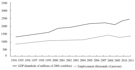
Source: Author’s own elaboration using data from Nicaragua’s Central Bank.
Graph 1 Nicaragua’s GDP and Employment
Even though all sectors have grown, they have done so at different speeds (mainly since 2000); agriculture has evolved more slowly while services have become the strongest sector in Nicaragua’s economy. As shown in Graphs 2 and 3, the relative contribution of agriculture and the manufacturing industry to the national GDP and employment has decreased, conversely to what is happening with the services. The agricultural sector’s lower contribution has been compensated for by the services sector.
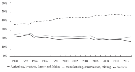
Source: Author’s own elaboration using data from Nicaragua’s Central Bank.
Graph 2 GDP share per Economic Activity.
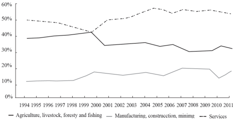
Source: Author’s own elaboration using data from Nicaragua’s Central Bank.
Graph 3 Percentage of Employment Generated by Economic Activity.
Something similar happened with exports, the traditionally highest-performing component of the agricultural sector1. Since 2006, as shown in Graph 4, the Nicaraguan agricultural exports began to grow at a lower rate than other exportable sec-tors, and they showed strong signs of less relative participation, placing them below the manufacturing industry.
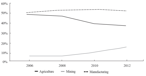
Source: Author’s own elaboration using data from Nicaragua’s Central Bank.
Graph 4 Percentage of FOB Exports per Economic Activity.
In relation to the above, this research focuses on identifying the determinant factors of Nicaraguan agricultural exports. As such, the paper can contribute by identifying the factors on which public and private policy must operate in order to help the sector regain its position and avoid future risk both for itself and for the Nicaraguan economy as a whole.
Nicaragua’s Export Situation
According to the World Bank (2012), Nicaragua’s average economic growth in the past decade (3.2% annual average) has been partially driven by an expansion in exports (average rate of 11% after 2000). Access to new markets, together with high international prices of some goods, has benefited the exports’ dynamism (WTO, 2012).
Although the exports from all the different sectors in Nicaragua’s economy have been growing over recent years, as shown in Graph 5, which presents a 6.2% aver-age annual rate of growth; agricultural exports have expanded the least. The mining industry is the sector that shows the highest annual average of growth (16.7%), followed by the manufacturing sector (6.3%), and then agriculture (4.3%).
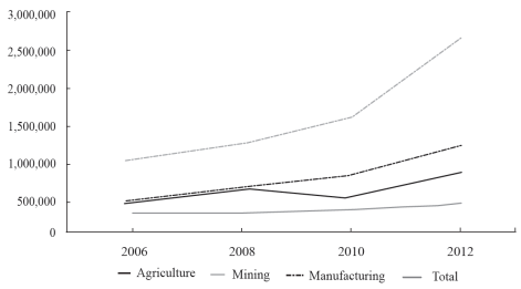
Source: Author’s own elaboration using data from Nicaragua’s Central Bank.
Graph 5 FOB Exports per Economic Activity in Thousand USD.
In terms of the exported products matrix, besides gold and cheese, no major changes can be seen over the last twenty years. Since 1995, the main products have been coffee, beef, sugar, and lobster. See Graph 6 for more details.
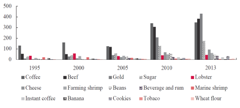
Source: Author’s own elaboration using data from Nicaragua’s Central Bank.
Graph 6 FOB Exports of Main Products in Millions USD.
Table 1 shows that, generally, exports have not presented significant fluctuations in terms of the country to which they are exported. The most important markets are: The United States, El Salvador, Honduras, Costa Rica, Canada, Mexico, Venezuela, and Guatemala. It can be seen that North and Central America are the most important destinations for Nicaraguan exportable products.
Table 1 Nicaragua’s Export Markets (percentages).
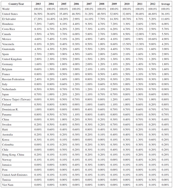
Source: ITC calculations based on UN COMTRADE statistics.
Since 1995, the situation for agricultural exports has not changed dramatically. During this time, a similar pattern can be seen to that of overall product exports. North America is the most important destination for these products (43.2%), followed by Central America (27.9%), Europe (14.8%), and South America (7.4%). Some minor exports are also registered for Asia and Africa, see Table 2.
Table 2 Nicaragua’s Main Agricultural Export Markets (percentages).
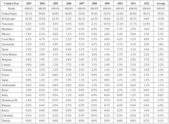
Source: Author’s own elaboration using WITS data.
In order to improve the performance of exports, Nicaragua has sought to strengthen relations with its current trading partners while continuing to look for new ones. This can be seen in the agreements the country has signed over the last decade (WTO, 2012), see Table 3.

According to The World Bank (2012), the FTA signed in 2005 between Central American countries, the Dominican Republic, and the United States (DR-CAFTA) played an important role in increasing exports. Exports to the US (Nicaragua’s biggest trading partner) have more than doubled since its implementation. More recently, Venezuela has also become more important and represents the second highest export destination. Despite some disadvantages regarding inefficiencies in its productive processes and its relatively poor performance in the world market, Nicaragua has a promising future if it maintains its current course. According to the 2012 reports from the World Bank and Economic Commission for Latin America (ELAC)’s forecast, Latin American exports will grow by 4%, meaning that Nicaragua will have the second highest growth rate with 13.5% percent, following only Bolivia (World Bank, 2012).
LITERATURE REVIEW AND THEORETICAL FRAMEWORK
To find out the determining factors of trade among countries, several researchers have implemented GMT. These models were first applied to international trade by Tinbergen (1962) and Pöyhönen (1963), who proposed that the intensity of trade relations between countries could be estimated relating economic concepts to Newton’s law of universal gravitation (an analogy). Thus, the volume of trade could be estimated as an increasing function of the national incomes of the trading partners and a decreasing function of the distance between them.
These models first became popular because of their perceived empirical success, but then due to lack of theoretical economic foundations, they started to be criticized. However, as time has passed, these shortcomings have been improved. This can be seen in papers including those written by Anderson (1979), Bergstrand (1985), McCallum (1995), Deardorff (1998), Anderson and Van Wincoop (2003) and Feenstra (2004).
A first basic form
As a starting point to understand GMT, it is necessary to review the relation between the law of gravitation and the economic concepts that allow us to estimate the volume of trade between countries. As explained by Reinert (2012) gravitational force between two objects (namely n and j), in equation form, is expressed as:

In the equation, the gravitational force is directly proportional to the masses of the objects (Mn and Mj) and indirectly proportional to the distance between them (Dnj). Thus, if it is expressed in terms of natural logarithms, what is multiplied is instead added and what is divided is instead subtracted. Formula (1) is thus transformed into the following linear equation:

According to Reinert (2012), the most solid theoretical foundations for handling mass consist in associating it with the corresponding national income of the countries that are to be included in a specific analysis. Moreover, the distance between objects is replaced by the distance between nations, and the gravitational force must be replaced by a variable that allows trade between countries to be measured.
Nevertheless, some authors such as Porojan (2001) and Kucera and Sarna (2006) incorporate the Gross Domestic Product per capita (GDP pc) into the GMT instead of using GDP as the proxy variable for national income. They adduce that is a better to estimate the purchasing power of nations. In addition, Lee, Koo and Park (2008) not only recommend including GDP pc in gravity equations, but also population data since higher income countries generally trade more due to the influence of their market size and superior infrastructure. Kalirajan (2007) and Iwanow and Kirkpatrick (2007) also considered population in their studies.
Thus, it is useful to define an initial form as follows:

Considering the Border Effects
Apart from these basic components, several authors, due to the presence of what trade economists call border effects2, consider that gravity models should include the effects political boundaries have on the relative prices of exportable products.
Over the last decade, the border effects have been incorporated into gravity equations in alternative ways. This was carried out by several authors following McCallum’s (1995) paper using the commonly applied concept of “remoteness”, which intends to reflect the average distance from a specific region to all its trading partners with the exception of the region where the trade is being measured3.
Several years later, in an attempt to continue to improve accuracy when considering border effects, Anderson and Van Wincoop (2003), as well as criticizing the theoretical simplicity of “remoteness”, developed the alternative concept of relative trade resistance. According to the authors, trade between two regions depends on the bilateral barrier between them relative to multilateral resistance (average trade barriers that both regions face with all their trading partners). In turn, this is incorporated as variables or indices, which are functions of all bilateral resistance (trade barriers)4 and the product of the respective price indices. This application has been recently further developed in works such as Baldwin and Taglioni (2006), Anderson (2011) and Martínez-Zarzoso, Voicu and Vidovic (2015).
Another option to border effects is a widely used alternative that consists in capturing price effects (including RER) between countries; a method that was used by Kandogan (2005), Thorpe and Zhang (2005) and Bahmani-Oskooee and Kovyryalova (2008). In order to add the border effects through the inclusion of RER in the GMT, a well-known procedure needs to be followed. The procedure begins with the transformation of the Nominal Exchange Rate (NER), calculated in United States Dollars (USD), into the NER expressed in Nicaraguan legal tender (USD is the most common currency in which the indicator is reported) and ends with the attainment of the RER between the Nicaraguan Cordoba (Nicaraguan currency) and the local currency unit of the J-eth country. For further details see Appleyard and Field (2003), Krugman and Obstfeld (2006) and Bahmani-Oskooee and Kovyryalova (2008). When choosing to add border effects through the RER, the model is expressed as follows:
A Final Theoretical Approach
Lastly, in order to give the basic model a more suitable approach to better represent commercial dynamism among countries, different authors have incorporated the effects of certain conditions by adding dummy variables. Some of these conditions and some of the respective authors who have considered them in their studies are the following: common language (Abedini & Peridy, 2008; Rose, 2000), FTA inking (Grant & Lambert, 2008; Longo & Sekkat, 2004), access to the ocean (Carrère, 2006), and geographical adjacency (Lampe, 2008; Lee & Park, 2007; Musila, 2005).
Finally, with regards to the model’s endogenous variable, the exports, as declared by Kepaptsoglou, Tsamboulas, Karlaftis and Marzano (2009), are the most common dependent variables found in trade flow gravity models and will therefore occupy the left-hand side of the equation.
The GMT in the Agricultural Sector
Despite GMT being more commonly used to describe the trading of manufactured goods, over recent years there have been many similarities5 when applying these kinds of models to agriculture; some examples can be found in Florensa, Márquez-Ramos and Recalde (2015) and Parra, Martínez-Zarsoso and Suárez-Burguet (2015). Even though these works pursue different aims, both separately represent the trading of agricultural and manufacturing products through the same theoretical specification that incorporates basic form variables, border effects (price resistance terms), and dummy additional variables. While the former studies the impact on trade for FTA agricultural and industrial products which came into force for ten Middle East and North African Countries (MENA), the latter analyses (for the same economic sectors) the effects of commercial agreements on the trade margins for eleven member-countries of the Latin American Integration Association (LAIA).
Nevertheless, it is important to note that due to complexities in trade policies, especially in the case of agricultural products, some authors such as Márquez-Ramos and Martínez-Gómez (2015) believe that the border effects treatment should be expanded. The authors generally call theses expansions trade preferences, which consider entry price systems, seasonal variations, and quotas or tariff-rates. Thus, to capture the relevance of these preferences granted to Morocco by the European Union6, the authors construct three exogenous variables that consider different perspectives that stem from the application of the agreements. The basis for the construction of these variables considers the estimation of the price reduction granted for Morocco compared with the entry price of the European Union’s most favoured trade partner for different products. Different ways to incorporate trade preferences in agricultural products are shown in Emlinger, Jacquet and Chevassus Lozza (2008) and Cardamone (2011).
However, for Nicaragua, it is not feasible to do so since there is no available information7.
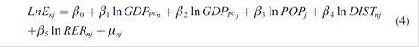
According to what is described above (in the Literature Review), and regarding data for different time periods (years), the resultant model to explain the Nicaraguan agricultural exports may be expressed as:
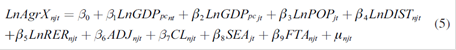
Where:
AgrX njt represents Nicaraguan agricultural exports to country j in year t
GDPpc nt is the Nicaraguan GDP pc in year t
GDPpc jt is the GDP pc of country j in year t
POP jt is the Population of country j in year t
DIST njt is the existent distance between Nicaragua and nation j in year t
RER njt is the RER between the Nicaraguan Cordoba and the local currency unit of nation j in year t
ADJ njt dummy variable that represents adjacency of Nicaragua with country j in year t
CL njt dummy variable that represents a common language between Nicaragua and country j in year t
SEA jt dummy variable that represents access to country j’s ocean in year t
FTA njt dummy variable that represents a FTA enforcement between Nicaragua and country j in year t
µ njt stands for the error term
The author recommends reviewing the work undertaken by Kepaptsoglou, Karlaftis and Tsamboulas (2010) for a well written summary of the most recent GMT research.
Based on the aforementioned work, the first hypothesis that this paper attempts to assess is the possible significant impact (positive or negative) that some general consensus factors have on Nicaraguan agricultural exports, such as the Nicaraguan GDP pc and a set of factors related to its trading partners. These include the GDP pc, the geographical distance that separates these countries from Nicaragua, the RER between the Nicaraguan Cordoba and the local currency unit, their population, the existence of geographical contiguity, the use of a common language with Nicaragua, and access to the ocean through ports. A second hypothesis to be tested is that the signing of FTAs has a positive effect on Nicaraguan agricultural exports and on the productive capacity of the sector.
METHODOLOGY
Data and Description of the Variables
Table 4 summarizes the description of the variable set used in this general model. The description of the variables includes symbol, name, units of measurement (or possible values in case of dichotomous variables), and the source for each component. It is important to note that ‘owning sea-ports’ does not appear as one of the variables in Table 4; it is a useless variable as all Nicaragua’s trading partners have sea-ports.
Table 4 Description of the Variables.
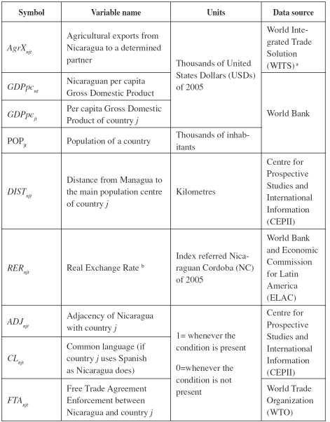
a This is an on-line system developed by the World Bank in close collaboration and consultation with various international organizations such as the United Nations Conference on Trade and Development (UNCTAD), the International Trade Centre (ITC), and the World Trade Organization (WTO).
b Calculated using an interaction of Consumer Prices Index (CPI) and Nominal Exchange Rate (NER).
Source: Prepared by the authors based on data from various sources.
The data used for this analysis is comprised of a total of twenty yearly observations (from 1990 to 2010) from twelve countries: eight have signed an FTA with Nicaragua and four have not despite being important trade partners. All twelve countries are among the sixteen main destinations for Nicaraguan agricultural exports.
The first group of eight countries consists of Mexico, the Dominican Republic, Guatemala, Honduras, El Salvador, Costa Rica, the United States, and Panama while the second group contains Germany, Spain, Great Britain, and Canada. The data used is made up of both time series and cross sectional data, which constitutes panel data.
Evolution of the GMTs’ Estimation Methodology
Over time, the GMT estimation methodology -in the quest for the most efficient estimates- has experienced many changes. The most common practice in the GMT’s empirical applications has been to transform the multiplicative model by taking natural logarithms and estimating the obtained log-linear model using OLS, which, according to Santos Silva and Tenreyro (2006), leads to biased estimates of the true parameters under heteroscedasticity.
Thus, the previously cited authors propose using a Pseudo Poisson Maximum Likelihood (PPML) estimation technique for cross-sectional data that is consistent in the presence of heteroscedasticity8. This provokes the first main change to the common practice and outlines Santos Silva and Tenreyro’s (2006) contribution as being highly influential despite criticism from authors such as Anderson (2011) and Márquez-Ramos and Martínez-Gómez (2015).
A second major contribution to the GMT’s estimation methodology was made by Baier and Bergstrand (2007). This work, based on findings from Baier and Bergstrand (2002, 2004) and Magee (2003), reveals that there are several plausible reasons to suggest that the quantitative effects FTAs have on trade flows using the standard cross-section gravity equation are biased. According to the authors, this is the case because the cross-sectional data approaches9 do not adjust well for FTA10 endogeneity11 since they are compromised by a lack of available suitable instruments.
Due to the previous, Baier and Bergstrand (2007) demonstrated that the most plausible estimates of the average effect that an FTA have on a bilateral trade flow are obtained using either panel data with fixed effects12 or differenced panel data with country and time effects, using OLS as an estimation method. For more detailed information about panel data techniques, the author highly recommends reviewing the following literature: Wooldridge (2002) and Gujarati (2003). According to both authors, these techniques are classified as follows: Constant Coefficients Models (CCMs), Fixed Effects Models (FEMs), and Random Effects Models (REMs).
Over recent years, the methodology to estimate GMTs has once again progressed: see Baier, Bergstrand and Feng (2011, 2014). The authors, apart from describing a process that is similar to Baier and Bergstrand’s (2007) to address the heteroskedasticity related to the endogeneity of the FTA variable, show arguably the best way to solve the residual autocorrelation (serially correlated errors and unit-root processes) that this variable could generate. To eliminate both problems, the authors propose estimating a theoretically-motivated gravity equation by fixed effects (FE)13, an equation that, according to Baier, Bergstrand and Feng (2011), must consider both a current and a lagged effect of the FTA variable. In Baier, Bergstrand and Feng (2014), the previously mentioned lagged effects of the FTA variable are replaced by a “random growth” model in differences14. Some applications of Baier et al.’s (2011, 2014) methodology, specifically for Latin American countries, can be seen in Florensa, Márquez-Ramos and Recalde (2015) and Márquez-Ramos, Florensa and Recalde (2015).
First Estimations of the Model
To detect eventual highly correlated exogenous variables (multicollinearity), we undertook a first estimation by using the simplest approach among panel data alternatives: CCM with OLS. The multicollinearity problem appeared and manifested itself through the wrong signs of the variables that were measuring the existence of a common language (with Nicaragua) and the enforcement of the FTAs Nicaragua - Mexico and Nicaragua - the Dominican Republic. Table 5 shows the expected signs of each variable’s coefficient and highlights the variables that are included in this first model’s estimation, which is shown in Table 6. The right sign could not be obtained.
Table 5 Expected Sign Between Nicaraguan Agricultural Exports and Independent Variables.
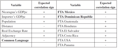
The expected correlation sign for FTA variables is obtained through descriptive statistics by comparing the flow of Nicaraguan agricultural exports before and after enforcement of the FTA.
Source: Author’s own elaboration.
Table 6 OLS Estimation in Presence of Multicollinearity.
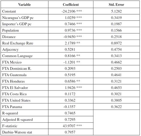
*** P < 0.01 ; ** P < 0.05 ; * P < 0.1
Source: Author’s own elaboration.
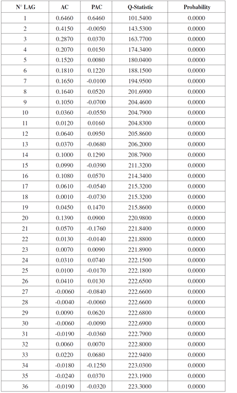
Subsequently, as shown in Table 7, once the highly correlated variables mentioned above were eliminated, the model was estimated again using CCM with OLS. However, due to the presence of heteroskedasticity and residual autocorrelation, as can be observed in Tables 8 and 9 respectively, another approach had to be found.
Table 7 OLS Estimation with Heteroskedasticity and Autocorrelation of Residuals.
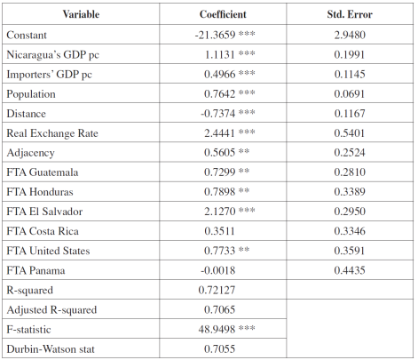
*** P < 0.01; ** P < 0.05; * P < 0.1
Source: Author’s own elaboration.
Table 8 Glejser Heteroskedasticity Test.
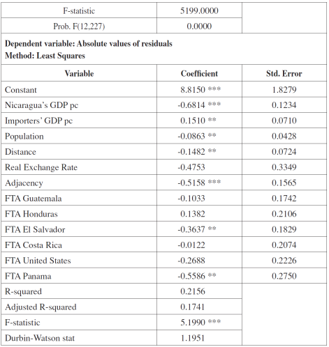
*** P < 0.01; ** P < 0.05; * P < 0.1
Source: Author’s own elaboration.
For this reason, we attempted to estimate the model by using the first version of the methodology described in Baier and Bergstrand (2007), which includes the use of panel data with bilateral fixed effects (country and time effects) and OLS.
Once again, a proper fit could not be achieved. That is because Baier and Berg-strand’s (2007) methods require new variables to be created to incorporate the country and time effects, which, in turn, created the new problem of multicollinearity15. This problem resulted in the application of any further approaches suggested by Baier et al. (2011), 2014 16 proving fruitless.
The Final Estimation of the Model
We attempted to estimate the model using different panel data methodologies and it did not achieve a proper fit both in relation to its forecast capacity and in regards to the significance of the exogenous variables.
Finally, we estimated the model using OLS and the Newey-West HAC consistent covariance estimator in order to improve the estimates of the coefficient variances. This procedure proposes a more general covariance matrix estimator, which, in the presence of heteroskedasticity and autocorrelation, corrects the estimates’ standard errors. This means that the Newey-West HAC covariance matrix estimator does not change the point estimates of the parameters, only their estimated standard errors (Newey & West, 1987). The Newey - West estimator is given by:

Where:
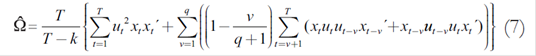
Where, T is the number of observations, k is the number of regressors, u t is the least squares residual, and q (the truncation lag) is a parameter representing the number of autocorrelations used in evaluating the dynamics of the OLS residuals u t .
To estimate the model, we used the EViews statistical software version 6.
RESULTS
The evaluation of the outcomes from the estimated model considers both the assessment of the global goodness of fit and the individual evaluation of the parameters. Table 10 shows the results.
Table 10 OLS Estimation with Newey-West HAC Procedure.
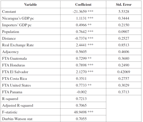
*** P < 0.01; ** P < 0.05; * P < 0.1
Source: Author’s own elaboration.
The criterion used, as a way of globally evaluating the beta parameters, was the F-statistic goodness-of-fit test, which indicates that the model can be used to make predictions17.
According to the p-values, we have found different results depending on the parameter. For the continuous variables parameters, the null hypothesis i = 0 is always rejected.
The Nicaraguan GDP pc, the GDP pc of partner nations, the population of these countries, and the RER show (through the positive sign of the related estimate) a positive correlation with Nicaraguan agricultural exports. These turned out to be significant (T227 = 3.232, p < 0.01; T227 = 2.310, p < 0.05; T227 = 8.428, p < 0.001 and T227 = 2.871, p < 0.01, respectively).
According to the distance, as indicated by the sign of the estimate and the related significance (T227 = -0.737, p < 0.01), the variable plays a predominant role in limiting the shipment of agricultural products from Nicaragua to other countries.
On the other hand, for the categorical variables parameters, the null hypothesis βi = 0 is not always rejected, which means that those variables do not achieve the necessary level to be considered as significant in order to promote or limit (depending on the sign of the related parameters) Nicaraguan exports. This occurs with geographical contiguity (T227 = 1.217, p = 0.225) as well as with some FTA variables.
The regression coefficients for the different FTAs that Nicaragua has signed possess both positive and negative signs18. For the latter, the sign would be contradictory because of the intention of having conducted agreements with those nations (at least for the agricultural sector). The former would be interpreted as a favourable influence of the FTAs over the dependent variable.
Based on the results in Table 5, Panama is the only trade partner that has negatively influenced the Nicaraguan agricultural exports in its market although this is not considered significant (T227 = -0.005, p = 0.9961).
Furthermore, the same outcomes presented in Table 5 indicate that the FTAs Nicaragua signed with Guatemala, Honduras, El Salvador, United States, and Costa Rica, have all been beneficial in terms of increasing the quantities of Nicaraguan agricultural products sold outside the country (Guatemala, T227 = 1.983, p < 0.05), (Honduras, T227 = 3.172, p < 0.01), (El Salvador, T227 = 5.056, p < 0.001), (United States, T227 = 2.553, p < 0.05), and (Costa Rica, T227 = 1.273, p = 0.2042). However, the significance level for the parameter related to the FTA signed by Nicaragua and Costa Rica is somewhat higher than 20%.
With this, the country markets of Panama and Costa Rica remain under an uncertain context. This is because the corresponding parameters do not reach the mini-mum significance level that would allow them to be classified as a trade-inhibiting FTA (Panama) or a trade-enhancing FTA (Costa Rica).
As suggested by Milner and Sledziewska (2007) and Sun and Reed (2010) 19, it is pertinent to comment that, in the present research, a complementary revision was carried out to determine whether the subsequent years presented a different situation. For this reason, new dummy variables representing the first three years after signing a given FTA were included in the analysis, and they were associated in several different ways in order to conduct new regressions. The results of the described attempt do not indicate any improvements for the significance level of any sub-period.
DISCUSSION
After reviewing the outcomes of the OLS estimation, it is reasonable to think that the proposed set of variables fulfil the study’s objectives.
The present research shows that there is a positive relation between Nicaraguan agricultural exports and the Nicaraguan GDP pc (1) as well as the GDP pc of Nicaragua’s trading partners (2). Similar results have been found by Martínez-Zarzoso and Nowak-Lehmann (2003) when GMTs are applied to asses Mercosur-EU trade. According to these authors, the positive influence both variables have on trade is due to the fact that the exporting party having a higher income suggests higher production levels, and the importing party having a higher income implies higher purchasing power.
However, according to some authors such as Grant and Lambert (2005), GDPs might have a less significant influence of on agricultural exports ( 1 and 2). They pointed out that in the case of agriculture, small income elasticity is to be expected mainly because this sector usually constitutes a much smaller percentage of national GDP than others such as the manufacturing sector. Another reason could be that when national income rises, countries may choose to trade higher valued non-agricultural goods.
The effect of Nicaraguan trading partners’ population on Nicaraguan agricultural exports (β3) resulted both positive and significant. According to Oguledo and MacPhee (1994) and Matyas (1997), population size is trade-enhancing since it promotes, among other characteristics, division of labour, specialization, and therefore economies of scale, which generate trade opportunities for both exporting and importing countries. A different perspective for this positive effect is revealed by Lee et al. (2008) who consider this variable as a proxy of market size. However, different perspectives such as Oguledo and MacPhee’s (1994) must be taken into consideration as they point out that population size could have a negative effect on trade. It could, therefore, be trade-inhibiting given that a large population may indicate large resource endowment, self-sufficiency, and less reliance on international trade: known as the absorption effect.
Regarding the distance (β4) between Nicaragua and its trading partners: a negative effect on the level of exports can be observed. Authors such as Egger (2002) and Pradhan (2009) have reached similar conclusions; the main reason being the association between distance and trade costs.
In this research, the findings point out that the impact of RER (β 5) on Nicaraguan agricultural exports is both positive and significant. The effects the RER has on international trade have been long studied and have shown different results. According to one approach, the results of which coincide with this research’s results, RER has a significant influence since it determines the relative cost of the products in the international market. In the same vein, Egger (2002), Cafiero (2005) and Kepaptsoglou et al. (2010) point out that local currency devaluation in real terms is beneficial for exports. According to the other approach, authors such as Bacchetta and Van Wincoop (2000) found that RER does not affect trade significantly because of its uncertainty.
Contrary to the most common results this research, geographical contiguity effects (β6) turned out to not be significant. Anderson and Van Wincoop (2003), Pradhan (2009) and Gul and Yasin (2011) came to similar conclusions. These results could be interpreted as a reflection of the loss of advantage that international land bridges have had in relation to the international seaports. Nevertheless, it should be highlighted that there is a widely accepted notion about the positive and significant influence geographical adjacency has on international trade. This is indicated by the evidence found in Boughanmi (2008), Masudur and Arjuman (2010) and Sun and Reed (2010).
Although the effects of a common language (β7) and having access to the ocean (β8) were not included in the model, it is useful to give an account of the evidence found in the literature about the positive and significant impact, that, in general, both variables have on exports.
Regarding common language, Montenegro and Soloaga (2006) found these results when estimating the impact NAFTA had on US-Mexico and US-third countries’ trade flows. The reason was either due to the ease of communicating in the same language or the cultural similarity between countries that share a language.
With regards to having access to the ocean, Limao and Venables (2001) have shown that a lower shipping cost is the main reason for positive effects on exports. The per-kilometre cost of land freight is far higher than the equivalent cost of shipping, which means that landlocked countries face higher transportation costs for foreign trade because of their lack of seaport facilities.
However, the author found divergent evidence when reviewing papers on the effects of FTAs. As pointed out by Kepaptsoglou et al. (2010) and Kohl (2014) -two important works that review the effects economic agreements have on trade flows- the performance of FTAs is still unclear. Some studies indicate trade creation and diversion while others indicate the opposite. Further evidence of this important discussion in the trade literature can be seen in Krueger (1999), Gilbert, Bora and Scollay (2001), Márquez-Ramos, Nowak-Lehmann, Herzer, Martínez -Zarzoso and Vollmer (2007) and Martínez-Zarzoso (2014).
To explain these divergent findings, although some authors cite different reasons, the most widely accepted are those related to the theories of comparative advantage. The most important are reviewed in Cuevas (2000), Krugman and Obstfeld (2006) and Raffo (2012). According to these theories, FTAs would benefit the commercial flow of relatively more efficient sectors at the expense of less efficient ones. Recent evidence supporting this idea, in the case of agricultural exports, can be found in Parra, Martínez-Zarzoso and Suárez-Burguet (2015).
Over recent years a complementary perspective has emerged that explains the divergent effects of FTAs. According to authors such as Kohl (2014) and Florensa et al. (2015), these effects depend on certain characteristics of trade agreements, such as their institutional quality and level of economic integration. These, in turn, offer insights into different types of FTAs. Moreover, the authors point out that the effects should be measured in terms of the “margins of trade”. The intensive margin (IM) is the increase in a country’s exports that result from maintaining and enhancing trade relations over time while extensive margins (EM) are related with the appearance of new products and markets. Hence, deeper integrated FTAs and better institutional quality should have more significant effect on margins.
For further reading on the effects FTAs have on trade margins, refer to the following studied: Hillberry and McDaniel (2003), Kehoe and Ruhl (2009) and Bensassi, Márquez-Ramos and Martínez-Zarzoso (2012).
Different results have been found depending on the country when measuring the effects FTAs (β9) have on Nicaraguan agricultural exports. Thus, it should be understood that signing an FTA only results in an increase in agricultural exports when the country or region is relatively less efficient than Nicaragua in the production of agricultural products and/or the FTAs’ institutional quality and level of economic integration are suitable. This is the case for Guatemala, Honduras, El Salvador, and the United States.
Furthermore, signing a FTA would result in a decrease in agricultural exports when the efficiency favours Nicaragua´s commercial partner, or because of the poor institutional quality and low economic integration within the FTA.
As such, the FTAs that have reported non-significant effects on Nicaraguan agricultural exports are supposed to be signed with countries or regions that have a similar relative efficiency in agricultural production and/or because the FTA’s institutional quality and level of economic integration are sub-standard (Costa Rica and Panama).
In terms of this last issue (when FTAs have reported a non-significant effect on Nicaraguan agricultural exports), there may be an alternative reason, which is related to the economic power of attraction that the US exerts over Nicaraguan goods. The strong trading relationship between the two nations cannot be denied, which may represent a kind of barrier to trade between Nicaragua and other countries. This could be the reason for the non-significant effects of those FTAs.
CONCLUSIONS
In summary, the most significant variables that increase the volume of Nicaraguan agricultural exports turned out to be the population of Nicaragua’s trading partners, Nicaragua’s GDP pc, the RER, and Nicaragua’s trading partners GDP pc. However, the variable distance turned out to be significantly trade-inhibiting. Moreover, the non-significant variables for Nicaraguan agricultural exports included geographical adjacency.
Finally, the effects FTAs have on Nicaragua and other nations depend on the particular country; different results were obtained in terms of statistical significance. It is necessary to mention that only in the cases of the FTAs that Nicaragua signed with Costa Rica and Panama should the hypothesis of a null impact on Nicaraguan agricultural exports not be rejected.
This allows us to deduce that, in recent years, the FTAs have improved the economic performance of Nicaraguan agricultural exports.
The main limitation this research had to face was the lack of information related to some of Nicaragua’s important trading partners. First, for the twenty years considered, there were some countries that despite being considered as one of the six-teen main trade partners with Nicaragua, there was no available information for the whole period, which meant that they were not incorporated in the study: two had signed an FTA (Taiwan and Chile) and two had not (Venezuela and Belgium).
It is also important to detail the effect that not incorporating some of Nicaragua’s trading partner’s particular features had on the final model. For example, it was not relevant to include owning sea-ports since the variable applied to all Nicaragua’s trading partners. Moreover, some exogenous variables presented a high correlation with other exogenous variables, which was expressed through a multicollinearity problem. These variables turned out to be, the common language between nations (Spanish), FTA Nicaragua - Mexico, and FTA Nicaragua - the Dominican Republic.
This research not only provides useful information for policy makers in the decision-making process, but also gives a methodological alternative to estimate GMTs when standardized procedures do not work properly and there are some data constraints. Furthermore, taking into account the complexities of trade policies (especially for agricultural exports), it is our opinion that further research about trade preferences20 should be undertaken as a way of incorporating border effects.

