English (pdf)
 Article in xml format
 Article references
 Send this article by e-mail
 Cited by SciELO
  Cited by Google
  Similars in
SciELO
Similars in
SciELO  Similars in Google
 Permalink
INTRODUCTION
The first decades of the 21st century have been full of contrasts for South America. After a process of sustained economic growth until 2012, fostered by the global rise in commodity prices, most of the economies in the region entered a phase of low or even negative growth, in a global context of low aggregate demand, the end of the "commodities supercycle", and a general worsening of global financial conditions, particularly for emerging countries.
In this context, the recommended economic policy from a Keynesian point of view would have been an increase in fiscal expenditures, accompanied by lower interest rates, in order to expand aggregate demand via the multiplier, which would lead to a boost in economic activity (Kalecki, 1954; Keynes, 1937).
However, South American countries' productive structure is characterized by combining a few highly competitive sectors, most of them based on natural resources, with a much less developed manufacturing industry -according to Diamand (1972), an "unbalanced" productive structure- which leads to a structurally high import elasticity. This hampers the implementation of expansionary policies in two ways: on the one hand, a stronger domestic market, with higher wages, would reduce competitivity and therefore curtail exports and increase imports, reducing income (Blecker, 2011; Hein & Vogel, 2008) and, on the other hand, the balance of trade deterioration would lead to an external constraint to growth, given the need of foreign currency in order to finance imports required for the productive process (Prebisch, 1950; Thirlwall, 1979). This characteristic of Latin American economies strengthened during the last decades after the abandonment of industrialization strategies that were prevalent until the 70s and the "reprimarization" of these economies during the recent commodity prices boom. Consequently, during recent years, many South American countries engaged in a "race to the bottom" by implementing austerity policies to reduce fiscal deficits, a fact that is illustrated by the recent return of IMF programs to the region in Argentina and Ecuador.
Conversely, it has been argued that the opposite approach (that is, a simultaneous and coordinated increase of fiscal expenditures) could be an alternative, more efficient strategy. This suggestion is based on the fact that, while one country's expansion would increase its imports, the simultaneous increase of its trade partners' economic activity would boost its exports, since they will require, at the same time, imported inputs. In this way, the total impact on the balance of trade would be lower.
Devising such a policy requires moving further away from the mainstream understanding of the relation between growth and trade, based on the calculation of trade elasticities (Houthakker & Magee, 1969), which focuses on exchange rates as the main adjustment mechanism, and, in more recent times, on DSGE models, which consider multiple countries that only differ in size (Corsetti, Meier, & Muller, 2010). Conversely, a Post-Keynesian approach, where the focus is put on production by considering income elasticities rather than on the exchange rate, allows a model to be developed that coherently integrates multiple heterogeneous countries.
The first step towards the development of such a framework was taken by Goodwin (1983) through the estimation of a "world matrix multiplier", which allowed the devising of, in Keynes' words (1936, p. 349), a "national investment program directed to an optimal level of domestic employment which is twice blessed in the sense that it helps ourselves and our neighbours at the same time". A particularly interesting feature of this methodology is that, while it takes a Keynesian standpoint by attributing a key role to aggregate demand, at the same time, it considers specific features for each country through their different import propensities, in line with a Harrodian (but also a structuralist) approach (Harrod, 1933; Prebisch, 1950).
Not much attention has been paid to this seminal paper, particularly due to the lack of consistent multinational data regarding growth and particularly trade. However, during recent years, multi-country databases (particularly inter-country input-output matrices) provided the required data for the implementation of these type of methodologies. This led to the Cingolani et al. (2013) work, which extended Goodwin's methodology by considering gross instead of net output and applied it to the countries in the Western Balkans, demonstrating that a coordinated expansionary fiscal policy is feasible for this region and displays better results for all dimensions (growth, trade, and fiscal costs) than an independent expansionary policy in each country. Portella-Carbo and Dejuan (2018) apply a similar methodology to the Eurozone to test if a Keynesian policy can promote not only growth but also income convergence, finding a trade-off between these two dimensions.
The South American region could also benefit from this approach in order to return to a growth path. This depends on a number of variables including: the multiplier effect of fiscal policies, the degree of productive integration among countries, and the dependence on extra-regional imported goods and services. A coordinated regional policy is viable not only because the involved countries display similar productive structures and face common challenges, but also because intra-regional trade displays, as opposed to extra-regional exchange (based on primary goods exports), a much more developed basket of goods and services, including a considerable percentage of manufactured goods and an important role for high and medium technology industries (CEPAL, 2018; Duran Lima & Lo Turco, 2010).
There is, however, a major challenge posed by the fact that South America shows much lower levels of productive integration than other regions such as the EU, North America, and Asia: it is divided between two major trade blocs (the MERCOSUR, composed by Argentina, Brazil, Paraguay, and Uruguay, and the Pacific Alliance, formed by Chile, Colombia, and Peru, plus Mexico from outside the region), and its main trade flows are not intra-regional but with external trade partners such as China, the EU, and the US. This implies that an expansionary fiscal policy, even if it is coordinated, might still have a considerable negative impact on the balance of trade.
The goal of this article is to implement the methodology developed by Cingolani et al. (2013) for South America, estimating inter-country matrix multipliers and then developing a linear program, which allows the necessary fiscal injection in each country to be calculated to allow for a positive rate of growth in all of them. This is done while maximizing "net gains", defined as the difference between GDP expansion and the increase in fiscal and external deficits.
The article is organised into five sections. After this introduction, the second section describes the current growth dynamics in the region and depicts regional trade. The third section of the paper presents the methodology to be implemented, and the fourth displays the main results. Finally, section five concludes.
AN OVERVIEW OF RECENT DECADES IN SOUTH AMERICA Growth
Dynamics and Fiscal Policy
The first decade of the 21st century was a period of extraordinary economic success for all countries in South America;1 they reached the highest rates of growth since the 70s. Between 2000 and 2011, the average GDP growth rate for the region was 3.9%, even taking into account the impact of the global financial crisis in 2009 (if this year is excluded, the average reaches 4.3%).
The expansion of economic activity was also accompanied by improvements in the labour market-generally not only limited to low unemployment rates but also leading to a reduction of informality rates (Bertranou, Casanova, & Sarabia, 2013; Saboia & Neto, 2018)-a more egalitarian income distribution and a strong aggregate demand, both domestic and external.
This period of solid growth was driven, schematically, by two main factors. On the one hand, the simultaneous election of progressist leaderships in most countries (known as the "pink tide") led to the implementation of policies that improved income distribution, such as increases in the minimum wage and social programs, and abandoned fiscal austerity, increasing domestic demand and (through the "accelerator") fixed investment (Kalecki, 1954; Samuelson, 1939).
On the other hand, the rapid increase in commodity prices, driven by a low but stable growth in developed countries, the emergence of new developing players such as China and, according to some authors, the use of commodities as financial assets (Belke, Bordon, & Volz, 2013; Carrera, 2018; Cheng & Xiong, 2014) had a twofold effect, increasing aggregate demand through higher exports but also relaxing the external constraint to growth by providing foreign currency in order to finance the increase in imports associated with a higher growth rate (Prebisch, 1950; Thirlwall, 1979). The external constraint to growth became even less binding during this period due to the low global interest rates and the consequent capital inflows into developing countries.2
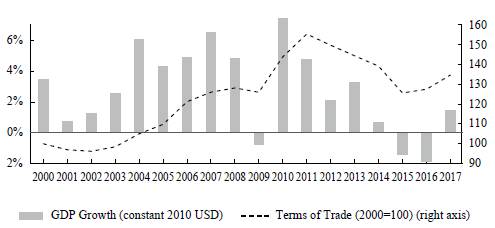
Conversely, changes in the external conditions after the financial crisis, often accompanied by the development of internal tensions, interrupted this virtuous growth dynamic: even though the region recovered quickly from the direct impact of the crisis in 2009, with a solid economic expansion in 2010 and 2011, growth rates have been low since 2012 and even negative for 2015 and 2016. A number of factors played a role in this drastic change in the regional dynamics.
First, the end of the commodity prices boom in 2014 led to an increase in the region's vulnerability (Abeles & Valdecantos, 2016): it implied not only a fall in aggregate demand but also a deterioration of trade balances, reducing the availability of foreign currency in order to finance the imported goods and services required to maintain high levels of economic activity. This has been particularly critical for the region since many countries "reprimarized" their productive structure (and, to even a higher degree, their exports basket) during the commodity boom (CEPAL, 2012). In some cases, the tighter economic conditions and the "defensive" reactions of firms and workers to currency depreciations in order to maintain their real income, led to an upsurge in distributional struggle, triggering inflationary processes.3
Second, the sudden reduction in availability of foreign currency could not be compensated for easily with higher indebtedness since capital lows were not as available as in the previous period due to a "fly to quality" process after the financial crisis of 2007/08. Therefore, the external constraint to growth expressed itself as a twofold effect, both real and financial. The accumulation of foreign reserves during the previous period and a widespread regulation of foreign financial flows provided some cushioning, which was more relevant in some countries than others (Ocampo, 2009).
Finally, a generalized political shift, particularly from 2015 onwards, implied the replacement of progressist governments by more conservative ones, which brought back the paradigm of "sound finance" for public accounts. Although fiscal deficits generally increased due to the fall in tax income, there were no strong fiscal expansions in order to countervail the lower activity in the private sector, both domestic and foreign; on the contrary, fiscal expenditure (especially investment) often reacted procyclically due to the application of austerity programs in order to recover fiscal balance.
The policy discussed in this paper, based on an expansionary fiscal policy, strongly contrasts with the ones implemented in the region in recent years. However, the success of such a strategy relies on the potential spillovers among countries. Therefore, an analysis of the structure of regional trade becomes necessary in order to discuss the potentialities and challenges of such a strategy. That is the goal of the next subsection.
Regional Trade
The simultaneous deterioration of trade balances after the end of the commodity prices boom was possible due to the fact that most of the trade for these countries is extra-regional: the main partners are the U.S., the EU, and China. Table 1 shows the trade flows of goods and services between the five considered countries, their main trade partners, and the rest of the world.
Table 1 Regional and Extra-regional Trade (2015) Billions of dollars
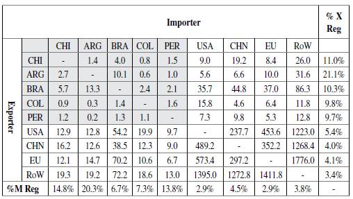
Source: Own calculation based on ICIO-OECD.
Indeed, the reliance on extra-regional trade partners is a feature of both exports and imports for the five considered countries. As shown in the last column of the table, the region is the destination for around 10% of total exports, the exception being Argentina, for which the region represents 21% of its external markets.
The analysis of imports depicts a similar situation although with higher divergences: countries such as Argentina, Chile, and Peru are more reliant on imports from the region (presented in the last row of the table), while Brazil and Colombia acquire foreign goods mainly outside the area. This feature is particularly manifest for final goods and services, while intermediate products are more frequently sourced in the region (particularly in the case of Argentina and Chile).
Regarding intra-regional trade, there are substantial asymmetries. Brazil is, by far, the most relevant regional player: it is the origin of 44% of the regional imports and the destination of 32% of the regional exports of the other four countries. Argentina is the second biggest player in the area, providing 27% of the regional exports and importing 28% of the regionally traded goods. Chile, Peru, and Colombia (in that order) explain the remaining trade lows.
In this regard, two main trade areas of the region can be identified, both structured around Brazil: one with Argentina and Chile and another with Colombia and Peru, which is considerably smaller than the previous one. In addition to these trade lows, Peru is also an important export destination for Chile.
These two features-dependence on extra-regional trade and internal asymmetries-have historically characterized the South American region. The (limited) regional trade has been fostered by the creation of two trade blocs: the MERCOSUR in 1991, which includes Argentina, Brazil, Paraguay, and Uruguay (Venezuela was a member, but it was suspended in 2016) and the Pacific Alliance (AP) in 2012, composed by Chile, Colombia, Mexico, and Peru. A boom in regional trade took place between 2004 and 2011, when trade lows grew at a yearly average rate of 20%, as shown in Figure 2. This strengthened regional integration, but without reverting the structural dependence on extra-regional markets: by 2011, when regional trade reached its historical record (84 billion dollars), trade with the rest of the world was 11 times higher.
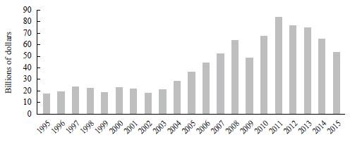
Source: Own calculation based on ICIO-OECD.
Figure 2 Regional Trade of Goods and Services (1995-2015)
Moreover, this trade pattern has strengthened during recent years: the slowdown in economic activity since 2011 came with a severe reduction of regional trade lows, which, after peaking at 83 billion dollars, fell to 53 billion in 2015, a 36% reduction in only four years. Although trade with the rest of the world also declined, the decrease was only by 17%, which reduced the importance of regional trade for the five considered countries.
This trade structure poses a constraint on the possibilities of devising a coordinated fiscal policy, given the fact that such a strategy will necessarily worsen trade balances since most international trade is extra-regional for the five selected countries. A generalized expansion in South America, without simultaneous growth in the rest of the world, will necessarily lead to a deterioration of the balance of trade of the region as a whole.
Therefore, a coordinated fiscal policy that also aims to be sustainable in the long run has to be accompanied by a strategic industrial policy able to develop supply capacity in the sectors with high extra-regional import propensity, such as electronics, transport equipment, mining, and basic metals in order to replace these purchases by regionally produced goods, which would strengthen crosscountry income-multipliers. It should be noted that, as was previously mentioned, regional trade displays a much higher participation of manufactured goods and high-tech industries than exports to extra-regional markets, implying that a coordinated fiscal policy would have a stronger effect for these sectors. Thus, there is a synergy between the short-term macroeconomic policy suggested here and an industrial policy oriented towards promoting regional structural change, which could be reinforced by directing the increase on public expenditure required to dynamize economic activity to specific industries.
After this depiction of the region's recent economic performance and its trade, the next section describes the methodology implemented to estimate a coordinated fiscal policy that, considering the aforementioned challenges, allows for generalized economic growth in South America, minimizing fiscal and external costs.
METHODOLOGY: ESTIMATING INCOME AND TRADE MULTIPLIERS FOR A COORDINATED POLICY
Matrix Notation and Remarks
In this section, matrix algebra will be used to present the calculation of net income multipliers, their balance of trade (BoT) effects and, finally, to develop a linear program in order to estimate an optimal coordinated fiscal policy. To facilitate the presentation of the methodology, it is necessary to first define some conventions regarding notation.
Vectors are represented by lower-case characters (e.g. z) and are always column vectors of dimension n x 1 (n is the number of countries) unless it is explicitly specified that they are transposed (e.g. z
T
). Matrices are indicated by upper-case characters (e.g. H), except diagonalized vectors (matrices with a vector on its main diagonal and zeros on the other cells), represented as lower case-characters with a hat (e.g.
 ). Vector e, of dimension n x 1, displays 1 as value on all its cells, and is used to be pre- or post-multiplied by other vectors and matrices in order to add them by column or row, respectively.
The methodology presented here is based on Cingolani et al. (2013). The only difference is that the rest of the world is considered as any other country, unlike in the original paper, where it is treated exogenously. The original methodology can be consulted in the aforementioned article.
Income Multipliers
The first step in order to estimate a series of cross-country income multipliers is to define a framework for production and trade that makes the interdependence between countries explicit, where both gross output z and trade balances b are represented. Such a framework can be formulated as:
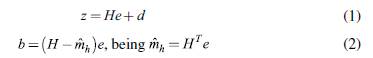
In expression (1), H is a matrix of dimension n x n (n is the number of countries considered), depicting intermediate and final production of goods and services, for domestic use in main the diagonal (h ), and traded with other countries in the off-diagonal cells (h ij , j # i). The only produced goods and services excluded from matrix H are the expenditures considered as exogenous, in this case, domestically produced public expenditures, included in vector d, of dimension n x 1. It should be noted that since input-output matrices depict primary income distribution, vector d only considers government purchases of goods and services (these include the provision of public administration services but not income transfers and subsidies).
Equation (2) presents the trade balance for each country, based on matrix H. Trade balances are calculated by adding the rows of the matrix (exports) minus the columns (imports), excluding the values from the main diagonal, which are production for domestic use. Vector d plays no role here since it only includes domestic demand components.
We can describe the system in "intensive" terms, that is, considering values per unit of gross output. In order to do this, we divide each column of matrices H and
 by the corresponding value of the vector z:

In this way, we can rewrite equation (1) in intensive terms, by replacing (3):

And solve for z:
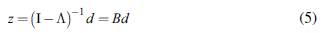
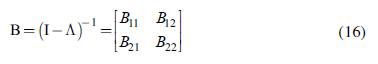
Matrix (I - Λ)-1, or B, is the equivalent of the "Leontief inverse" for our multi-country setting. As such, the cross-country interdependence is made explicit since the gross output of each country will be determined by the values of the exogenous final demand d in all others. With the first-difference estimator (5), we obtain:
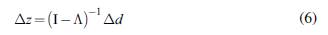
Matrix (I - Λ)-1 also represents the inter-country gross output multipliers: each cell (I- Λ)-1 ij describes the increase in country's i gross output when there is an increase of 1 monetary unit in exogenous demand from country j.
From the income side, we can also represent gross output as the sum of intermediate inputs x and value added y:
Again, we can describe the system in intensive terms, by defining
 , that is, the proportion of intermediate inputs in gross output per country:

And, finally, solve z:
Equation (9) shows that gross output is defined as the total requirements generated by value added y. Combining expressions (5) and (9), and by taking the first differences, we obtain:

Therefore П is the net income multipliers matrix, which describes the rise in total net income (value added) caused by an increase in exogenous demand d. Each cell in the main diagonal (П ii ) represents each country's income multiplier, while the off-diagonal values (П ij ,i # j) describe the increase in a country's i net income for an increase of one monetary unit in country's j exogenous demand.
As such, the total net income of a country is determined by the level of autonomous expenditures in all countries (including itself), making the fact explicit that output determination is not a national but a simultaneous, worldwide process. Moreover, we can divide expression (10) for each country into two components: the income generated by domestic autonomous expenditures and the one created due to other countries' exogenous expenditures:
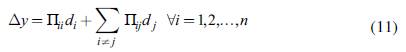
However, since our objective is to estimate a coordinated fiscal policy for a certain group of countries (in this case, the ones from the South American region, which we will call "group 1"), it is necessary to distinguish between intra-regional and extra-regional income multipliers. This means separately considering the effects of an increase in autonomous injections in group 1 countries or in group 2 ones. In order to do this, we can rewrite the output, income, and trade systems-that is, equations (1), (2), and (7)-as partitioned matrices:
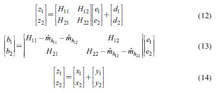
Analogous to expression (3), we can define partitioned matrices in intensive terms:
And, as in equation (5), matrix B = (I - Λ)-1 is also partitioned:
Then expression (5), which determines gross output, can be rewritten as:
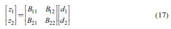
We can also rewrite the income multipliers from equation (10), distinguishing between intra-regional and extra-regional autonomous demand and their effects:
Finally, since we are focusing on group 1 countries, we can assume Δd 2 = 0. Then, the effect on group 1 countries of an increase in autonomous demand in these same countries is:

This expression will later be fundamental as part of the linear program to estimate the optimal fiscal policy since it provides the net income multipliers for the region.
Trade Balances
In order to estimate a fiscal policy that considers BoT effects, it is necessary to also understand the effects that changes on autonomous demand have on trade balances for each country. Starting from equation (2) and introducing (3), we obtain:
This shows how trade balances are understood as fully determined by output levels z. Naturally, the sum of trade balance
 equals zero since trade is a zero-sum game where one country's exports are another's imports. Replacing (5) in (20) and taking first differences, we obtain the effects of each country's balance of trade for a change in autonomous demand Δd:

However, and as was the case for income multipliers, we are interested in distinguishing between BoT effects due to changes in autonomous expenditures in each group of countries. Therefore, by replacing the expressions from (15) in equation (20), we can describe trade for each group of countries. Intra-regional trade in each group of countries is:
While extra-regional trade can be defined as:
The total BoT for each region is simply the addition of its intra-regional and extra-regional balances:
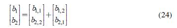
Given that trade is a zero-sum game, both intra-regional trade balances are zero, and the sum of group 1 extra-region BoT is the inverse of group 2 extra-region BoT:
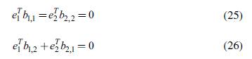
By replacing expression (17) in (22), we obtain intra-regional trade balances as a function of autonomous demand:
It can be seen that intra-regional trade balances do not only depend on autonomous demand from countries in the same group; they also depend on the other group of countries' demand. This responds to the fact that part of that extra-regional demand requires imports from the region (directly or indirectly), which, in turn, implies the supplying country must import other inputs, part of which originate in the region.
Similarly, we can write extra-regional trade balances by replacing (17) in (23):
Once again, the extra-regional BoTs depend on both regional and non-regional autonomous demand. Because we focus on group 1 countries and we disregard intra-regional balances of trade, we have to focus on expression b l 2 while assuming d 2 = 0 in order to know the effect an increase in domestic demand has on extra-regional balances of trade:
This expression will be a key input in the estimation of the optimal fiscal policy, since it represents the effects of such a policy on the extra-regional BoT for each country, which is one of the constraints for the feasibility of such a strategy.
A Linear Program for a Coordinated Fiscal Policy
Once the income multipliers and the BoT effects of an increase in autonomous demand (here, public expenditure) are known, it is possible to develop a fiscal policy that allows for an increase in net output with a limited impact on the fiscal stance and the balance of trade. In order to do this, we develop a linear program, which implies the optimization (maximization or minimization) of a linear function, subject to a number of constraints.
In our framework, the variable to optimize (in this case, minimize) will be the total fiscal expansion required by group 1 countries (the region). There are three constraints: first, that the percentual increase in GDP has to be higher than a defined value
 (in our case, 1%) for all countries in the region; second, that the change of fiscal expenditures has to be positive for all group 1 countries; and third, that the fiscal injection must lead to "net gains" π, understood as the increase in GDP minus its "costs": its impact on the government's budget and on the balance of trade. This final constraint can be written as:
Replacing equations (19) and (29) in (30), and after some algebraic manipulation, we can rewrite equation (30) as:

The way this optimization is specified is not irrelevant, given that it defines the goals of our policy. Indeed, these equations hide some important theoretical and practical implications that should not be overlooked. One of these issues is that our definition of net gains, following that of the original paper, includes the policy's impact on the government's budget. However, from a Keynesian point of view, the relevance of fiscal deficits can be discussed. An alternative target could be the attainment of full employment in all countries instead of a specific growth rate. This could be done by estimating the required increase in gross output to provide jobs for the currently unemployed population based on a linear employment function. Another option could be to maximize regional growth assuming that each country has a specific limit for increasing its BoT deficit (for example, assuming limited credit on international markets, a loan from international institutions or, in a Bretton Woods fashion, the chance for funding a limited balance of payments deficit).4
Another implication of the way we define our system of equations is that, by assuming an equivalent rate of growth for all countries as the policy goal, there is no treatment of the current income gaps, which would not necessarily be reduced. Indeed, Portella-Carbo and Dejuan (2018) find a trade-off between growth and convergence in a similar study for the Eurozone. Thus, a policy that aims to reduce the income differences among South American countries should explicitly include this goal in the optimization. Due to space constraints, this will not be addressed in this paper, but further research into this issue would complement the approach presented here.
Considering the three aforementioned constraints, based on equations (19) and (31), the linear program to minimize the fiscal expenditure can be written as:
As a result, we obtain a vector Δd 1 * which displays the minimum fiscal injection required for each country to at least achieve the require d growth rates that are subject to the described constraints. We can use vector Δd 1 * to compute the effects of such a policy. First, we can calculate the resulting rates of growth, from equation (19):

And the intra and extra-regional effects on the BoT, based on equations (27) and (29):
By replacing the values obtained in equation (30), we obtain the net gains of such a policy:

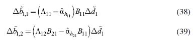
Finally, and as a key policy decision, we can compare the coordinated fiscal policy and its effects with an independent policy by each country. The latter is understood as the individual fiscal expenditure required by each country to attain the same rate of growth if its partners do not increase their current fiscal expenditure. If we define a matrix β with the main diagonal of matrix B 11 , the required independent fiscal expansion Δd 1 can be calculated as:
And the corresponding effects on the balance of trade, like in equations (34) and (35), are:
Therefore, the corresponding net gains of an independent fiscal policy would be:

It should be noted that while the net gains of a coordinated fiscal policy do not include the intra-regional trade effects Δb
*
1,1
, the independent fiscal policy does consider them (
 ). This is because the sum of such effects is necessarily zero, which makes them irrelevant when the unit of analysis is the region as a whole (which does not deny that intra-regional compensation mechanisms might be necessary). Conversely, when each country is concerned exclusively with its own BoT, they have to be kept into account.
A fundamental policy decision will be the comparison between the net gains of a coordinated fiscal policy (π*) and the ones corresponding to an independent expansion (π). The next section will present the estimated income and trade multipliers of South America and the impacts and net gains of both a coordinated and an independent fiscal policy in order to provide a basis for comparison.
A COORDINATED FISCAL POLICY FOR SOUTH AMERICA
To perform the analysis of income and trade multipliers and to estimate an optimal fiscal policy, the database we used was the inter-country input-output (ICIO) matrix developed by the OECD, covering the 2005-2015 period. It includes 64 countries plus a "rest of the world" (RoW) region.5 The five countries included in the South American region are Argentina, Chile, Brazil, Colombia, and Peru. This presents some limitations to the estimations since other relevant countries from the region are excluded due to lack of data. However, in 2018 these five nations represented 89% of the South American GDP measured in PPP according to the IMF (2019).
While the input-output matrix contains data for 36 sectors in each country (presented in the previous sections) these have been aggregated in order to calculate income and trade multipliers, obtaining a matrix H of dimension 65x65 for each year, with data on goods and services production and trade. Domestic government expenditure was considered as the exogenous source of demand, while all other final demands were considered endogenous and, therefore, part of the H matrix.6
By aggregating the matrix to a country level, we miss the chance of analysing the sectoral impacts of our policy, and, consequently, to direct government expenditures to specific sectors since they are considered at an aggregate level in this paper. Further studies including a sectoral dimension could refine the policy we suggest by computing a vector of fiscal expenditures that fosters demand for specific sectors, with the more ambitiuos goal of promoting not only growth but also structural change.
For the sake of brevity, most results are only displayed for the last year of the series (2015). Table 2 presents the income multipliers for the region in 2015, calculated following equation (19). Each cell describes the effect of an increase of one monetary unit in government expenditure of the originating country (column) on the receiving country (row). The diagonal values (in bold) show the national income multipliers. The highest national multiplier is displayed by Argentina, followed by Colombia, Brazil, and Peru, while Chile displays a much lower value than the rest of the region.
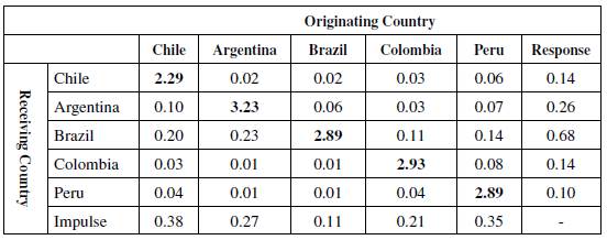
The column "Response" adds the total effect on each country if its four regional partners increase their public expenditure by one monetary unit. Conversely, the "Impulse" row represents the total cross-country effect of an increase in government expenditure by the same amount. It can be seen that the country that most benefits from a generalized fiscal expansion would be Brazil and, in a second place, Argentina, given their roles as providers of inputs and final goods for the region. Conversely, a fiscal expansion in Chile and Peru would trigger the greatest income effect for their partners. This poses a challenge for the development of a coordinated fiscal policy since countries whose expansion implies higher spillovers onto the others are those who benefit the least.
If we consider the addition of both coefficients as a measure of regional importance, in the sense that a higher value represents a more relevant role for the determination of regional output, we can say that Brazil (0.79) is the most relevant country, followed by Argentina (0.53), and then Chile (0.52). Conversely, Colombia (0.45) and particularly Peru (0.35) play a less relevant role.
In order to estimate an optimal fiscal policy, it is necessary to also know the effects in the balance of trade of a fiscal expansion in each country, presented in Table 3, which uses equations (27) and (28). Each cell shows the effect that a fiscal expansion of one monetary unit by the country in the column has on the impact on the balance of trade of the country in the row. The diagonal describes the effect of a fiscal expansion by each country on its own BoT. Naturally, all these values are negative since a fiscal expansion and its multiplying effect increase imports barely affecting exports.7 Less integrated productive structures, such as Colombia, Chile, and Peru show higher import requirements and, therefore, a strong negative trade effect of an expansionary fiscal policy, while Argentina and Brazil have lower impacts on their BoT. It should be noted that these values are not per dollar of GDP but per monetary unit of fiscal expansion (the corresponding effects on GDP were presented in the previous table).
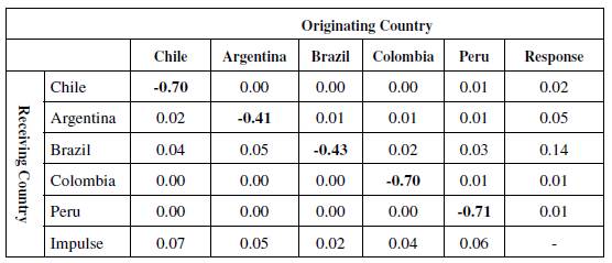
The "Response" column describes the total effect on each country as a result of an expansion of the other four. Again, Brazil is the country that benefits the most, improving its BoT by 0.14 monetary units if the other four considered countries increase their fiscal expenditures by one monetary unit each. It is followed by Argentina and Chile.
The "Impulse" column presents the total effect on the trade partners' BoT of an increase of one monetary unit in the fiscal expenditure of the column country. In this case, the most relevant countries are Chile, Argentina, and Peru. Therefore, the same regional asymmetry exists: while Brazil's balance of trade benefits greatly from an expansionary policy, given its key productive role in the region, it does not cause much exports from the region, given the fact that it mainly imports from extra-regional countries.
Considering both results, we can devise an optimal fiscal policy according to a linear program (32) that implies an expansion of GDP of at least 1% in the five considered countries and leads to net gains, as defined by equation (31). The effects on growth and the BoT, as well as the increase in government expenditure, are calculated following expressions (33), (34), and (35). Table 4 presents the details of this policy. The first column shows the effect that the fiscal expansion has on each country's GDP. In 2015, it was possible to carry out a fiscal policy leading to the minimum required GDP growth, which is 1% for all countries.
The second column shows the required expansion in fiscal expenditure in order to achieve the specified rate of growth. The countries having to deal with a higher fiscal effort (in terms of their current expenditure) are Chile and Peru. In all cases, the required expansion shows reasonable values that are lower than 3% of 2015 government expenditures. However, when the distribution of the total fiscal expansion is considered (column 3), it can be seen that Brazil and Argentina, given the size of their economies, undertake most of the fiscal effort. It is positive that Brazil, which, as previously shown, would be the main beneficiary of this policy, is also the most committed country from a fiscal point of view, which aligns incentives among countries.
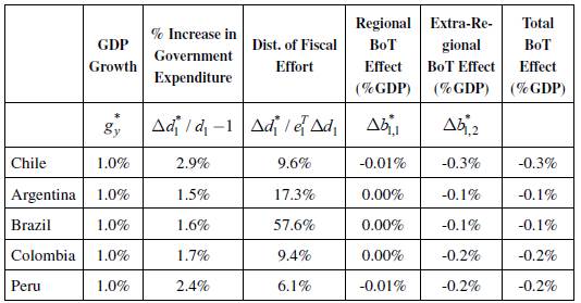
Finally, the last three columns describe the effects in the balance of trade. The regional effect in trade (that is, the effect on each country's BoT only with the other region members) is negligible, and, naturally, it adds up to zero since one country's exports are another's imports. The extra-regional effects, however, are higher and negative, particularly for Chile, Colombia, and Peru, which worsen their trade balance by a margin between 0.20% and 0.25% of GDP per percentual increase in income. However, except for Colombia, these countries are currently the ones with better trade balances, facilitating the implementation of this strategy.
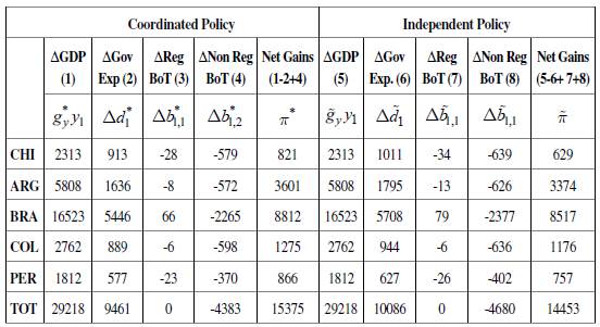
The key policy variable is, however, the net gains of a coordinated fiscal policy (defined as the difference between the increase in GDP and the "cost" of the policy in fiscal and external balances) and its comparison with the gains of an independent fiscal policy that would lead to an equivalent rate of growth. On the one hand, the result of linear program -equation (32)-, and equations (33), (34), (35) and (36) show, for a coordinated fiscal policy, the resulting GDP growth, the required increase in government expenditure, the impact on the regional and extra-regional balance of trade, and the net gains. On the other hand, equations (37), (38), (39) and (40) present the same variables for an independent fiscal policy that leads to an equivalent rate of GDP growth. Table 5 compares the effects of both policies for 2015.
Table 5 Comparing Coordinated and Independent Fiscal Policies (2015) Millions of dollars
Source: Own calculation based on ICIO-OECD.
It can be seen that the required fiscal expansion in order to achieve an equivalent GDP growth is lower for all countries when a coordinated strategy is implemented, and the effect on the balance of trade is less detrimental. The difference is particularly important for Chile, Peru, and Argentina, and smaller for Colombia and Brazil. The latter contrasts with our previous results: even though Brazil is the country that has received the most benefits at an intensive level (per unit produced) the size of its economy implies that regional trade is a relatively small part of its total exchange, and, therefore, its gains are also of limited importance for the country.
Despite these differences, net gains are higher for the five considered countries when a coordinated strategy is implemented than when an independent fiscal policy is applied; this calls for regional coordination. Moreover, and as shown in Table 6 (which presents the percentage difference of the net gains of a coordinated and an independent policy for each year), this has been the case for the five countries during the whole period under analysis (2005-2015).
Table 6 Net Gains Differential of Coordinated and Independent Fiscal Policies (2005-2015)
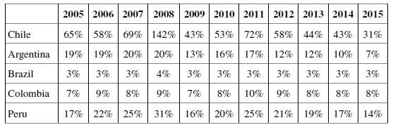
Source: Own calculation based on ICIO-OECD.
This differential, that can be understood as an incentive for cooperation among countries, generally shows an upward tendency until 2011 (excluding 2009), and, since then, it starts reducing considerably. This is consistent with the slowdown in regional trade after 2011 (weakening the cross-country multipliers) and the fall in commodity prices, which tightened the external constraint to growth. However, net gains always remained higher for a coordinated policy than for an independent one, indicating that the former would yield better results than the latter.
CONCLUSIONS
Since 2012, growth rates in South America have been low, with some countries even facing sharp recessions. In a context of stagnant global demand, fall of commodity prices and risk-averse global financial markets, fiscal austerity has only made the situation worse by curtailing aggregate demand.
However, austerity is not completely irrational from a national point of view: in a context of falling exports and, therefore, shortage of foreign currency, a fiscal expansion would probably increase economic activity, but this would lead to higher imports and, therefore, to a disequilibria in balance of payments.
This article presented a policy proposal that would allow this limitation to be overcome, at least partially, based on the methodology developed by Cingolani et al. (2013). By estimating inter-country fiscal multipliers and making use of linear programming, we have shown that a coordinated fiscal expansion between five countries-Argentina, Brazil, Chile, Colombia, and Peru-can lead to an increase in GDP for all of them, with lower impacts on the governments' budget and the balance of trade than an independent policy. This result is explained by the fact that, while one country's expansion would indeed increase its imports, part of these purchases would come from the region, implying a positive effect on its partners' growth and balance of trade.
However, it has been shown that the regional productive structure and international relations in South America pose several challenges for such a policy: limited regional trade (with high dependency from extra-regional partners, particularly China, the U.S., and Europe), weak coordinating institutions and high asymmetries between countries imply that carrying out a coordinated expansionary policy would not be exempt from tensions. Indeed, the political feasibility of such a policy is not granted, considering the very different approaches to regional integration of the two main trade blocks in the region (on the one hand, a more inward-looking MERCOSUR, and, on the other hand, a Pacific Alliance which aims to increase extra-regional exports). There have also been recent attempts by the regional political leadership to promote trade agreements with extra-regional partners, particularly the MERCOSUR-EU deal and the potential Brazil-US agreement.
Notwithstanding the above, our results showed that a coordinated strategy is better than independent actions both on the fiscal and the external front for all countries, with reasonable values: in order to achieve a 1% GDP growth in all countries, the required fiscal expansion for each one of them would range between 1.5% and 3%. Moreover, the two countries required to make a larger effort relative to their current spending, Chile and Peru, are the ones that currently display lower fiscal and trade deficits, which reduces potential regional tensions. However, putting compensation mechanisms in place or facing certain public investment projects through regional banks could increase incentives for these countries.
Despite these positive results, our analysis comes with a warning: given the dependence of all countries on extra-regional imports, an expansionary policy (even coordinated) implies a worsening of the trade balance for the region as a whole, and particularly for Chile, Colombia, and Peru. This is not an exclusive South American feature, but the constraints are higher for the region given its trade patterns and disintegrated productive structure, which poses a limit to the achievable rates of growth for such a policy. In order to overcome these limits, an industrial policy seeking to reduce technological dependency (in which the increase of fiscal expenditures should take part, targeting specific sectors) becomes necessary in order to allow for structural change and long-term growth, an issue which should be tackled by further research.
It should also be noted that the growth target defined (1% of GDP for the five countries), as well as our definition of "net gains" (GDP growth minus the increase in fiscal and trade deficits) are somewhat arbitrary. From a Keynesian point of view, an alternative goal could be to achieve full employment, without particular concerns for fiscal deficits. Finally, the issue of convergence among countries is not discussed here but cannot be ignored. The flexibility of the presented framework would allow for the implementation of all these additions and improvements; the foundations for its computation have been laid in the previous sections, and future research should go along this path.
To summarise, a coordinated fiscal policy is not only feasible, but it would also lead to considerably better results than independent initiatives by each country. Industrial policies to enhance integration could increase the potential of this strategy. Unfortunately, most South American countries are taking the opposite path by cutting their fiscal expenditures and undermining regional agreements. The outcome is visible and discouraging: South America has been the region with the lowest growth rates in the world for the last five consecutive years. The results presented in this article show that austerity is not the only option, and that it is time to discuss expansionary fiscal policies in order to return to a growth path.