Inglés (pdf)
 Articulo en XML
 Referencias del artículo
 Enviar articulo por email
 Citado por SciELO
  Citado por Google
  Similares en
SciELO
Similares en
SciELO  Similares en Google
 Permalink
Inequalities in income, health and education, (perhaps) will continue to increase
until they become unpredictable and politically intolerable (...) and will thus fuel individual opportunism. Each person's wish will be to progress alone; individualism will legitimise and strengthen inequalities. Jaques Attali (1999)
INTRODUCTION
In 1958, Alban Phillips established a seemingly stable and negative relation between nominal wage inflation and the unemployment rate for the case of the United Kingdom (1861-1957). Subsequently, Samuelson and Solow (1960) tested it for the U.S. (1934-1954) and since then -with multiple changes- it has become widespread and has been incorporated into the Keynesian theory. Henceforth it would be known as the Phillips Curve (PC). Since then, it has become a powerful theoretical instrument used to explain price formation and define economic policy. However, since Friedman (1968, 1977) and Phelps (1968) incorporated the adaptive expectations hypothesis, its comprehension has evolved drastically, and presently it remains a central piece in modern macroeconomic debate.
Since the 1980s, the macroeconomic consensus, which has derived from the rational expectations revolution, has been progressively establishing itself in the New Classical Approach (NCA) and, successively, within the New Keynes-ian Approach (NKA).1 Both schools of thought consider inflation stability to be essential for the sound functioning of the macroeconomic system. Specifically, the NKA -the integrated version of Carlin and Soskice (2015)- acknowledges the existence of an Accelerationist Phillips Curve (APC), along which the economy moves around its medium-run full equilibrium.
During the Great Moderation (Stock & Watson, 2002), in the developed countries, the focus of monetary policy turned to establishing monetary rules and constrained discretion, along with fiscal rules that would maintain macroeconomic fundamentals aligned and, as a result of its "economic success", inflation stopped being a recurring issue in the developed economies (Blanchard, 2008), but remained so in the emerging world. In economies, such as the case of Mexico, said processes have not vanished, and have always been a topic of broad discussion and controversy in the implementation of monetary policy.
As a result of the 2009 Great Recession, the developed world focused its interest and its theoretical and economic policy concerns on deflation, but in countries such as Mexico -on the contrary- inflationary spikes were observed, reason why the problem of inflation and the trade-off with labour variables have remained fundamental both for the authorities and for the academy.
For the U.S., Romer and Romer (1989) showed that reducing inflation inevitably leads to recession and unemployment. Shortly after, Ball (1993) suggested the sacrifice rate, which measures the unemployment gap and the output gap that should be generated by stabilising monetary policy in order to decrease inflation and return the economy to its long-term path. The sacrifice rate is a quotient, in which the numerator represents the observed unemployment and output deviations with respect to their natural or potential levels, and the denominator represents the change in inflation of the final period with respect to the initial one. This allows to algebraically measure the change in the gaps with respect to a one-point change in inflation.
For the case of Mexico, considering a brief analysis of the last five decades, we can see that, following a short period of stability and growth (1958-1970), it has been characterised by systematic processes of instability and the corresponding macroeconomic adjustments. Since the early 1970s, when macroeconomic fundamentals began to misalign, Mexico has had an important inflationary tradition. Between 1973 and 1999, the economy went through frequent stagflation processes in which it on average exhibited double-digit inflation rates, except for 1986 and 1987, in which these spiked to 130%, on average, and with the exception of 1993 and 1994 as well, when these marked 7-8%. Only after adopting the Inflation Targeting Regime (ITR) in 2001 (Ramos-Francia & Torres, 2005), did the Mexican economy register systematic one-digit inflation, although on many occasions it was above the central bank target.
The last important inflation hike was observed in the second half of the 1990s. First, in 1995, in the wake of the greatest economic and financial crisis since the 1930s Great Depression, inflation attained 52%, and shortly afterwards (in 1998), as a result of the crisis in Asia and South America, other important inflation outbreaks were registered. Nonetheless, from then on inflation has decreased progressively until, as a result of both the macroeconomic congruence and the Banco de Mexico's autonomy, the country started registering annual inflation rates around 3%.2
Since 2001, subsequent to the implementation of the ITR, inflation has been low and stable. However, we have identified that since 1998 there have been six important disinflation episodes, which have been associated to negative output and unemployment gaps,3 which are consistent with conventional theory, Romer and Romer (1989) and Ball (1993).
Nevertheless, at least since 2005,4 precariousness5 and informality in the labour market -which since then and up to 2019Q4 have affected, on average, over 12% and 56% of the employed population, respectively- are the variables that mainly absorbed the costs of disinflation policies and which have, thereby, become a major problem of the Mexican economy, a bigger problem than the unemployment rate.6
This article demonstrates that, in accord with modern conventional theory (NKA), the Banco de Mexico has managed to dissipate inflation episodes by generating slack in labour markets and in economic activity, and the main adjustment variable has largely been the RCLC,7 thus increasing precariousness -more than unemployment-, which has importantly affected the quality of life of a large share of the population, therefore, strongly affecting social fabric and cohesion.
In order to prove this, we estimated 6 models of the New Keynesian Phillips Curve (NKPC), (four with OLS and two with ARDL)8 for 2005Q1-2019Q4, the only period for which integrated and consistent official series are available. Likewise, we made an in-sample forecast in order to choose the model that best explains the monetary policy impact on labour market variables in Mexico.
We found short and long-term robust statistical relations between slack in economic activity (as measured by output gaps, unemployment gaps and labour precarious-ness) and corrective monetary policy, contrary to what could appear to be intuitive, the Labour Informality Rate (LIR) does not cointegrate with the disinflationary adjustment.
The paper is divided as follows. Following the introduction, we review the theoretical issues and literature regarding the sacrifice rate concept. In the next section, we analyse stylised facts concerning the variables of interest, and after we present econometric issues, along with the estimates that substantiate our hypothesis. Finally, we conclude and make some final remarks and further comments.
THEORETICAL ISSUES AND LITERATURE REVIEW
Consistent with the NKA -that we here identify with Ball et al. (1988), Gali and Gertler (1999), Mankiw (2001), Blanchard (2008), Lanchard et al. (2010), and principally Carlin and Soskice (2015)- in the event of an inflationary shock, the central bank adjusts (raises) the interest rate, which lowers aggregate demand and, consequently, modifies businesses' supply function with the consequent effect of reducing labour demand and labour costs, which we here define as the relation between average productivity and average real wages in manufacturing. Thus, in this theoretical and economic policy approach, the cost of inflation stabilisation falls finally and inevitably on producers, who react by adjusting their labour costs in two ways: by reducing the workforce (by decreasing working hours and/or the number of personnel) and/or lowering wages, including nominal wages.9
In the first case, the adjustment impact is mainly reflected in a higher unemployment rate. In the second case, with higher labour precariousness choices will depend on the degree of labour flexibility.
Romer and Romer (1989) clearly documented that those disinflationary processes in the U.S. (1920-1987) were always caused by a tight monetary policy that affected unemployment, albeit only temporarily.
This argument was strengthened shortly afterwards by Ball (1993), who related this effect for a broad range of developed and emerging economies. He mentions that recessions in the U.S. between 1961 and 1988 mainly derived from a (tight) disinflationary monetary policy and he argues regarding the effectiveness and the consequences of the aggressive nature of the policy with reference to what is best for a central bank: either to reduce inflation gradually (gradualist monetary policy) or do it abruptly (Cold Turkey). He found that in terms of social welfare it is better to distribute losses throughout more periods, using the first approach. What remains unclear in this methodology is which one works better in the medium term.
Mankiw (2001) mentions that the inflation-unemployment trade-off is undeniable, at least in the short run, but it is necessary for a price formation theory. He questions the validity of the NKPC since it relies heavily on backward-looking expectations. Despite the backward-looking expectations assumption that could restrict the microeconomic foundation of the PC, Gali et al. (2001) prove that for the Euro area a backward-looking Phillips curve is efficient in order to understand inflation dynamics. Loria et al. (2020) applied it for México.
Carlin and Soskice (2015, pp. 476) contribute to this discussion stating that policy makers should opt for the most efficient policy, that is, the one that succeeds in minimising economic losses, and they do so by measuring the sacrifice rate derived from the NKPC. They mention that it is necessary to observe the type of relationship between inflation and unemployment in order to determine which strategy is more efficient and they conclude that, if the NKPC is linear, in the medium term, the same deviations result in unemployment and in output using either (gradualist or shock) strategy.
Different articles analyse inflation determinants and their impacts on the economy. Andersen and Wascher (1999) study the evolution of the sacrifice rate in developed economies in a context of low inflation. Gonçalves and Carvalho (2008) show that countries that adopted the ITR had to sacrifice 4% less output in order to reduce inflation by 1% as compared to countries with other monetary policy frameworks. More recently, Borio and Gambacorta (2017) analyse the case of developed countries, showing that monetary policy loses its effectiveness insofar as the nominal interest rates approach zero. For the U.S., Cecchetti and Rich (2001) find that the cost of reducing inflation by 1% is between 1 and 10% of real production in annual terms, and Fuhrer (1994) presents a similar result, where it is necessary to sacrifice between 0.56 and 6 points of the GDP. Both show that this indicator is appropriate to assess the monetary policy impact.
For the case of Mexico (2002-2019), Loria et al. (2020) estimated an NKPC in order to calculate the sacrifice rate in terms of the unemployment rate and -as with Romer and Romer (1989)- they did not find permanent effects on that variable caused by stabilising monetary policy. Therefore, they concluded that, since the adoption of ITR in 2001 (Ramos-Francia and Torres, 2005), monetary policy has been efficient in making unemployment rates and inflation rates stationary, and they did not find robust empirical evidence, which would relate stabilising monetary policy to structural changes in the GDP and in the unemployment rate.
In general, we can say that, as a consequence of the macroeconomic success of the Great Moderation (1985-2008), most developed economies lost interest in the sacrifice rate hypothesis.
Although the worldwide consolidated NKA textbook by Carlin and Soskice (2015) recognises the importance of the sacrifice rate, it clearly defines the main concern of the developed world regarding the Zero Lower Bound problem that threatened them between 2009 and 2012, and once again during the corona crisis.
However, in emerging economies, such as in the case of Mexico, the key macroe-conomic problem continues to be that of recessions and depressions accompanied by inflation processes, reason for which we sustain that, for this type of countries, the sacrifice rate hypothesis and its proper management by the authorities is still extremely relevant.
Mexico has implemented changes in its monetary policy since 1995, in order to slowly approach the inflation targeting scheme (Turrent, 2007). First, it left behind the fixed exchange rate regime, to move to a floating one, granting broader margin for the central bank to act. This generated a series of depreciations of the domestic currency, causing agents to doubt that the Central Bank would be able to meet the goal of controlling inflation. To achieve its objective, the Banco de Mexico created various policies throughout the period, such as el corto which consisted of withdrawing liquidity from the money market by controlling the money balances of commercial banks. It was not until 2008 that the Central Bank finally adopted the interest rate as its main instrument (Ramos-Francia & Torres, 2005). For example, for 1996-1998, the monetary base growth targets were published for the first time in the National Official Gazette (Diario Oficial de la Federación), to give certainty to the market and to anchor inflation expectations. However, this instrument was not effective.
In 2000, the first step was taken to formalise the inflation targeting scheme, since it was expressly announced that the Banco de Mexico was committed to achieving a 3% inflation target in the long run. Since then, the Mexican economy has enjoyed single-digit inflation rates.
Ramos-Francia and Torres (2008) set forth three reasons the study of inflation using the PC in Mexico is relevant. First of all, the inflation evolution is different from that observed in the developed countries, as it shifted from three-digit levels in the 1980s to one-digit levels starting from 2000. The second reason is that, by using it, it is possible to analyse the role of expectations (adaptive or rational) in the inflation dynamics. Finally, this curve facilitates the study of disinflationary processes.
More recently, Ashley and Verbrugge (2020) attest that for the U.S. the PC has not weakened and that the coefficients of the model are stable and offer accurate conditional recursive forecasts.
In this regard, this article focuses on assessing the sacrifice rate of the Mexican economy since 2005 as a consequence of said disinflationary processes, but the difference is now in evaluating said costs not only in terms of the unemployment rate, but also - and this is our main contribution- in terms of the strong increase in precariousness in the Mexican labour market for 2005Q1-2019Q4.
STYLISED FACTS
Following a long recession in the 1980s, unemployment in Mexico increased, but not as much as in other (Latin American and OECD) countries, given that a number of compensatory mechanisms operated, such as migration abroad -particularly to the U.S. - and informality, see Figure 1.10 Despite a long period of slow growth recorded by the Mexican economy since 1982, the unemployment rate never exceeded 6%, even considering the years in which depressions were observed, such as 1983 (-6.8%), 1995 (-6.3%) and 2009 (-5.5%).11
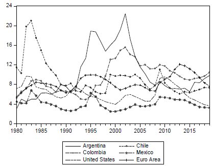
Source: Author's own calculations based on IMF (2020).
Figure 1 Unemployment rate in various countries, 1980-2019
A second analysis (Figure 2) for a shorter period and with quarterly series (2005Q1-2019Q4) would suggest that since 2009 inflationary reduction has mainly decreased with the rapid increase in the RCLC and RW.
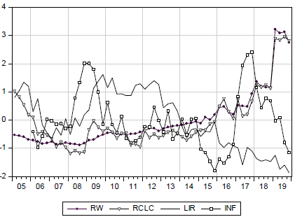
* To be visually comparable, the data were normalised by the following statistical procedure  where X is the arithmetic mean and a is the standard deviation.
Source: INEGI (2020).
Figure 2 México: RW, Labour Precariousness, Informality and Inflation, 2005Q1-2019Q4. Normalised Data*
This figure is highly relevant, given that it shows important structural changes in the Mexican labour market. With the onset of the 2009 Great Recession, the LIR and the RCLC started to grow notably.
Everything seems to indicate that the 2012 labour reform12 contributed to generating permanent changes in at least three senses: a) formal employment13 grew in a manner unseen since public records began, given that, while in the period 19932012 the average growth rate of formal employment was 2.55%, after that reform (and until 2018) it grew by 3.64%. But the most paradoxical aspect is that in the first period, the GDP increased by 2.29%, and in the second by 2.17%, which yields elasticities of 1.11 and 1.67, respectively; b) at the same time, the LIR fell abruptly reaching its lowest historical levels, and c) precariousness (RW and the RCLC) grew exponentially.
Therefore, it seems clear that the disinflationary adjustment mechanism was reducing labour costs -by increasing labour precarity- and not reducing occupation or increasing unemployment and informality.14
When there is either an economic contraction or growth slows down, firms negotiate different labour conditions with workers, in order to reduce Unit Labour Costs (ULC). Consequently, two things can happen: a) firing employees and/ or b) cutting wages and also reducing (or even increasing) working hours. It is plausible to assume that these negative macroeconomic conditions force workers to make their working conditions more flexible (precarious).15 We found statistical (negative) significance between economic growth and the RCLC (r = -0.49, t= -4.11), and Granger causality (up to 4 lags) running from economic growth to the former, and not inversely.16 Figure 3 shows that since 1998, but more clearly since 2012, potential GDP growth has been declining, reason why corporate sales and incomes are likely to decrease too. Therefore, the above mechanism tends to apply.
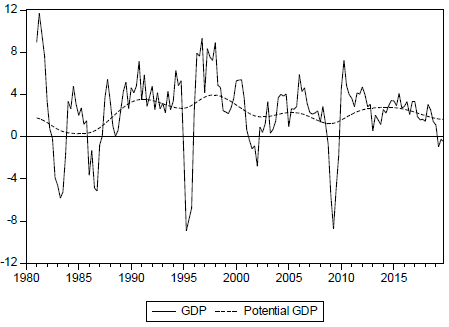
Source: INEGI (2020).
* Potential GDP was calculated with the HP filter (Hodrick & Prescott 1980).
Figure 3 GDP growth rate (observed and potential*), 1980-2019. Normalised Data
When analysing the quarterly ULC of Mexican manufacturing (MULC), a strong downturn in trend can be noted between 2001 and 2016, which can reflect the above-described firms' adjustment mechanism, and the surprising increase from that year onwards can be accounted for by wage increases decreed by the federal government, see Figure 4.17
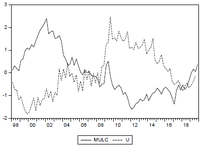
Source: Author's own calculations based on INEGI (2020).
Figure 4 Manufacturing sector unit labour costs and unemployment rate, 1998Q2-2019Q4. Normalised Data
Thus, the increase in MULC, in the unemployment rate, and in labour precarious-ness can be explaining the decreasing trend in aggregate demand, particularly of private consumption,18 reason why an additional important long-term recessionary effect could be generated.
There is an extensive discussion regarding the effects of monetary policy on the real sector of the economy. Moreno-Brid and Ros (2009) mention that by concentrating only on price stability the Central Bank has diminished investment rates in physical capital, thus, reducing gross capital formation and long-run growth. Perrotini (2007) and Huerta (2006) claim that there are effects of monetary policy on economic growth that ultimately are reflected in the labour market. Loria et al. (2019) and Loria (2020) agree with the previous arguments, however they conclude that according to robust econometric tests of structural change the monetary policy has not had any permanent effects on potential output or on the labour market for 2002Q1-2018Q2.
In addition, because the Banco de México adopted its ITR, it sets the interest rate and since it has no management on the monetary aggregates, changes in the interest rate modify the money market equilibrium and loanable funds market, affecting output and labour markets. Our results implicitly demonstrate that workers' wages are affected during disinflationary periods, due to considerable increases in the RCLC.
However, we believe that the monetary policy has been efficient in reducing inflation, not in recovering wages, because that is beyond its responsibility. According to theory, the distortions generated in the labour market cannot be corrected by the Central Bank. Institutional (supply side) policies are necessary for this purpose.
On the other side, for 2005Q1-2019Q4 there is strong statistical evidence that monetary policy has not been destabilising because when Δ = 0, it has been guaranteed that U
G
=Y
G
=
0. This means that when the Central Bank maintains stable inflation (at its target level), unemployment and output are at their natural levels, as can be seen in Figure 5. Nevertheless, labour precariousness is a consequence of the new adjustment mechanisms in which firms have benefited from the flexibilisation of the labour market, where the Central Bank has no acting capacity.
= 0, it has been guaranteed that U
G
=Y
G
=
0. This means that when the Central Bank maintains stable inflation (at its target level), unemployment and output are at their natural levels, as can be seen in Figure 5. Nevertheless, labour precariousness is a consequence of the new adjustment mechanisms in which firms have benefited from the flexibilisation of the labour market, where the Central Bank has no acting capacity.
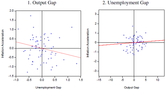
Source: Author's own calculations based on INEGI (2020).
Figure 5 Scatter plot with a linear fit, 2005Q1-2019Q4. 1. Output Gap
Given the characteristics and concerns expressed in this article, we evaluate the sacrifice rate in the labour market in terms of gaps in unemployment and the RCLC, and not only in the output gap. To that end, it is necessary to first present selection and identification criteria for disinflationary episodes and the methodology for their estimation.
For our purposes, there is a disinflationary episode during which the inflation trend falls substantially; that is, when it starts at a local maximum and ends at a local minimum. More precisely, and following Ball (1993), a disinflationary episode occurs when the inflation trend is negative for over four consecutive quarters and when inflation decreases by over 2%. This definition ensures its correct identification because the episode does not conclude with a small rebound in inflation, and, in addition, it is associated with episodes prompted by disinflationary monetary policy, which distinguishes them from small fluctuations caused by short-term shocks unrelated to the labour market.
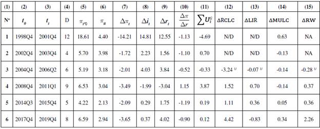
We detect six distinct disinflationary episodes between 1998Q4 and 2019Q4, as shown on Table 1. All of them share regularities, except for episodes 1 and 4, which correspond to unique circumstances. The first one is extraordinary, since it corresponds to a correction of an important inflation outbreak, during which two-digit figures were observed, and which is associated to relevant nominal exchange rate depreciations (16%), which are accounted for by economic and financial crises in Asia and in South America.19 On the other hand, the specific nature of episode 4 corresponds to the 2009 Great Recession that also caused important nominal depreciations (21.1%), combined with a strong decrease in economic activity.
Table 1 Disinflationary episodes, 1998Q4-2019Q4
Note. “t
0
” is the initial observation and “t
t
” is the final one; “D” measures the episode duration in quarters; “i” is the nominal interest rate of the 28-day Mexican Treasury bonds (CETES) and “r” is the real interest rate; Δ is the change rate;  measures the efficiency of the monetary policy;
  is the manufacturing sector unit labour costs, where W
t
is the real average wage of manufacturing, L
t
is the number of manufacturing workers, and Y
t
is manufacturing output; RW measures the proportion of employed people who receive up to 1 minimum wage compared to those who receive up to 5 minimum wages.
is the manufacturing sector unit labour costs, where W
t
is the real average wage of manufacturing, L
t
is the number of manufacturing workers, and Y
t
is manufacturing output; RW measures the proportion of employed people who receive up to 1 minimum wage compared to those who receive up to 5 minimum wages.
1 / Due to information availability, the change rate is between 2005Q1 and 2006Q2.
NA: Not available.
Source: Author’s own calculations based on INEGI (2020).
To characterise each one of these disinflationary episodes in terms of our hypotheses, we present their main features:
All episodes, except for the first one, are characterised by having variations in inflation between -1.72 and -3.65 percentage points (column 7).
Column 10 shows the monetary policy efficiency insofar as it reports the inflation decrease generated by the increase in the real interest rate. In that sense, in all cases the stabilising monetary policy has been efficient, despite relatively low inflation levels,20 particularly in episode 5 and, moderately, in episode 6. In all cases, a correct sign is registered, except for episode 4, which refers to the Great Recession.
It is observed that efficiency was diminishing clearly and progressively over the first three episodes; which could be explained by the hybrid policy used by the Banco de México at that time. In its 2008 Report (Banco de México, 2008), the Central Bank declared that it would start using the bank funding rate as an operational target instead of the "corto". That change seems to have been adequate given that in episode 5 efficiency increased notably.
In all episodes, except for episode 4, there were relevant increases in nominal and real interest rates (columns 8 and 9). In the first one, it is observed that, given the inflation peak in 1998, the nominal rate (CETES) rose from 19% to 35% during one year, which contributed to an increase in the real interest rate from 3.54% to 16.09%, this being the highest figure of the entire analysis period. As already noted, episode 4 is extraordinary given that the inflation correction, to a large degree, can be attributed to a strong decrease in aggregate demand that occurred as a consequence of the Great Recession. In that sense, although inflation was high in 2007, the negative impacts of the Great Recession on aggregate demand prompted the adoption of anticyclical monetary and fiscal policies. As mentioned above, episode 1 stands out because of the aggressive nature of the monetary policy. During the remaining disinflationary periods, the stabilising policy was more moderate given that its efficiency improved and that inflation outbreaks were weaker.
However, episode 6 -which is more recent, and which continued until 2019Q4- exhibits the highest initial inflation over the last 5 periods, only lower than the first one. The variation of the real interest rate is also the highest, only below the first one.
Only episode 4 reports a reduction in interest rates, which could be due to a non-conventional countercyclical monetary policy (Quantitative Easing) which was adopted by the Banco de México, as in the other central banks. In addition to said measures, the central bank increased the real monetary base to GDP by almost 18% between September 2009 and April 2010, to later resume its average growth rate of approximately 5.7%.
Another fact worth noting is that the sacrifice rate, measured in terms of the unemployment gap (column 11), declined from 3.87 to 0.12 between episodes 4 and 6, while the RCLC variation was the highest, column 12.
Column 14, in turn, shows the change in the MULC in each disinflationary episode. Leaving aside episode 1 -which is completely atypical-, episodes 2, 3, and 4 exhibited important reductions. However, starting from episode 5, the disinflationary cost, measured by Δ RCLC and by Δ RW, has been the highest in the entire period of analysis.
In the last episode -as mentioned above- what stands out is the strong increase in the MULC, which can explain the fact that the cost of disinflationary adjustment has mainly fallen on the precarious labour conditions that we use here.
ECONOMETRIC ISSUES
To prove the central hypothesis of this work, we estimate six Phillips Curves augmented with the RCLC and the LIR: four with OLS and two with ARDL, as a result of which, in principle, we face the problem of "alternative or rival models" to explain inflation. However, in no case do we have contradictory results. On the contrary, we find that all results point in the direction of our main hypothesis.
In order to distinguish and select the model that best proves our hypothesis, we employ the following strategy: a) the results must comply with statistical criteria of correct specification; b) the results should show regressor signs as dictated by the theory (Hendry and Richard, 1983), c) that, in accordance with different common statistical indicators of contrast, the in-sample forecast should yield smaller values, Pindyck and Rubinfeld (1991, pp. 336-341), and d) that "the interocular trauma test" of Kennedy (2002) is passed.21
Although these six estimated models are NKPC versions, only the first four are accelerationist, given that the autoregressive parameter (which refers to adaptive expectations)22 is statistically equal to one;23 however, the fact that the other two models are not accelerationist does not invalidate the analysis or its comparison.
For exposition purposes, we divide what follows into two subsections.
ACCELERATIONIST PHILLIPS CURVES (APC)
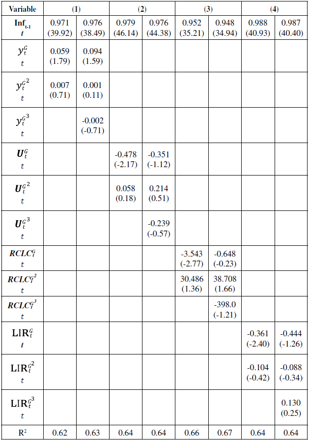
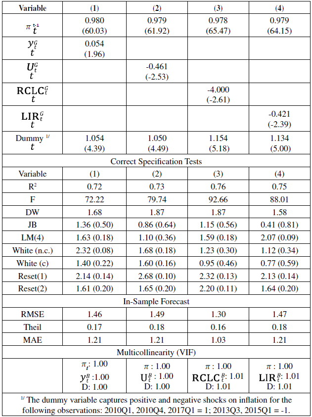
As a first approximation to our hypothesis, we estimate four alternative models that explain the inflation dynamics in Mexico for the entire period. The first two include only the output and unemployment gaps, and the last two, only the RCLC and the LIR gaps.24
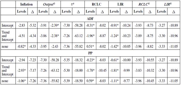
Given that all variables used in this section are stationary (see Table A1 of the Statistical Appendix) OLS is appropriate since it ensures that the estimated parameters are consistent, unbiased and efficient (Hayashi 2000, p. 52). Table 2 shows the statistical results of the first four models.
All models are correctly specified, the goodness of fit (R2) is acceptable and similar in all cases, the signs are as expected by the theory and point in the direction of our hypothesis, and non-linearities were ruled out, see Table A2.
The estimated parameters suggest that inflation is mainly sensitive to the RCLC gap, marginally to the unemployment gap, and, finally, to the output gap.
In accordance with the in-sample forecast accuracy indicators, model (3) better explains the inflation dynamics, which suggests that the RCLC is the variable that, to a greater extent, has assumed the cost of inflationary adjustment.
PHILLIPS CURVES AUGMENTED WITH LABOUR PRECARIOUSNESS
In this section, we estimated two Phillips Curves augmented with the RCLC in levels, which when expressed in this way, are unit roots. Given that the series have different integration orders (see Table 1A)25 we applied the ARDL method (Pesaran & Shin, 1998; Pesaran et al., 2001).
These models are OLS regressions that include lags, both in the dependent variable and in explanatory variables (Greene 2008, pp. 571), and gained popularity in examining cointegration relations among variables of a different integration order, not higher than (Nkoro & Uko 2016, pp. 64 ).
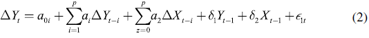
If y t is the dependent variable and x 1 ,..., x k are k explanatory variables, a general ARDL model (У ,х 1 ,…,х к ) is represented as follows:
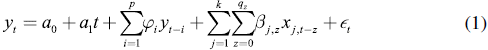
Where α 0 is the constant, and α1,φ1, and ß j,z are the coefficients associated to a linear trend, lags of yt and lags of k regressors x j,t , respectively for j = 1,... ,k, and Є t are Gaussian type innovations (Pesaran and Shin 1998, pp. 372).
Following this general formulation, three very important complementary representations can be made for analysis and inference purposes. The first is typically used for intertemporal dynamic estimation; the second, for the long-term (cointegration), and the third gives the long-term form in its representation of the conditional error correction (CEC), Pesaran et al. (2001).
Table 3 presents short-term estimations using this technique. Unlike the four previous models, we observe that the autoregressive term -despite being high- is lower than one, showing a high intertemporal persistence of inflation expectations, and it also fully validates the NKPC.
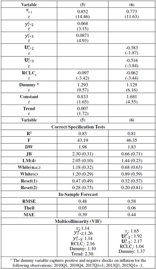
We found that the first lag in the output and unemployment gaps is not significant, which can be due to the fact that the adjustment in the labour market due to inflation takes effect after two quarters.26 The number of lags was chosen in accordance with Akaike's minimisation criterion.
ANALYSIS AND DISCUSSION
Based on the results of the six models, we find the following important regularities:
OLS models (1 to 4) are NKPC versions, and are expressed in terms of gaps, which, given their specification, only have simultaneous effects. Of all of them, the one that stands out is the one with the highest value of the RCLC gap and the lowest one is that of the output gap. This would suggest that inflation is a lot more sensitive to adjustments in labour markets than to those in production.
Using the VIF test, it is proved that no model incurs in collinearity, reason why the parameters are significant, and the signs are correct.
Models 5 and 6 -given their nature- estimate simultaneous and dynamic effects, which allows to see the temporality of adjustment more accurately. In the same way, they incorporate a dummy that captures inflation and disinflation (transitory) shocks, by means of which serial correlation, normality and heteroscedasticity are also corrected.
The output and unemployment gaps27 have adequate signs and are significant with 2 and 3 lags, which would indicate that inflation takes between 6 to 9 months to decrease after the adjustment in the real sector, as a consequence of the stabilising monetary policy. Specifically, it is noteworthy that 9 months later the effect in both cases is a lot greater, particularly with respect to the unemployment gap, which reinforces the hypothesis that it is upon the labour market where the weight of the macroeconomic adjustment mainly falls.
We find that all Phillips Curves are linear,28 reason why it is suggested that both a gradualist and an abrupt (Cold Turkey) policy adjustment generate the same losses.
In models 5 and 6, the RCLC is contemporaneous, statistically significant and has the correct sign, which, unlike the previous variables, shows its immediate disinflationary effect. We left out the LIR since it was not significant, something that we forewarned.
Although model (6) does not yield the highest R2, or the lowest in-sample forecast, it is the one that generates better short-term economic results in terms of our hypothesis and, therefore, we focus our analysis on it. Again, this model explains that the weight of stabilising monetary policy mainly falls on the labour market, given that the inflation decrease is based on widening the unemployment gap and on increasing the RCLC. Although the accumulated effect of two and three lags in the first variable on inflation is 0.9 and that of the RCLC is only 0.06, as we will see in the next section, in which we measure long-term effects, it turns out that the cost of adjustment in terms of the RCLC is higher according to the sacrifice rate.
To confirm the existence of long-term equilibrium relations (cointegration), we applied the Bound F-test of Pesaran et al. (2001) and Pesaran and Shin (1998), which verifies if the coefficients δ1 and δ2 are different from zero.
The null hypothesis (Ho) of the F test suggests that the coefficients of the long-term relation variables are equal to zero and it contrasts with two critical values that are known as the lower bound and the higher bound. The critical value of the lower bound assumes that all series are stationary, and, therefore, the cointegration issue vanishes. On the other hand, the critical value of the higher bound assumes that the series have a unit root.
If the calculated statistic exceeds the bands, a conclusion can be drawn without having to prove the integration order of the variables. If the estimated F is lower than the lower bound, the null hypothesis cannot be rejected, and a long-term relation is ruled out. On the other hand, if the calculated value falls between both bounds, the test is inconclusive. Finally, if the value is higher than the upper bound, the null hypothesis is rejected, and it is concluded that there is a stable long-term relation (cointegration) among variables.
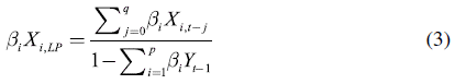
According to Nkoro and Uko (2016, pp. 83-84), long-term parameters result from the following expression that takes the estimations of short-term parameters from Table 3:
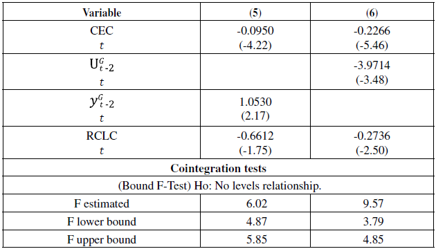
Results from Table 4 show that for short-term estimators there are corresponding long-term representations, all of them having broad statistical and economic sense. However, and in the interest of this paper, model 6 allows to evaluate the sacrifice rate in terms of the labour market, in addition to yielding the highest error-correction parameter.
Finally, Table 5 presents the summary of the results of models 2, 3, 5 and 6 in terms of estimating the sacrifice rate.
The estimated slopes
(βxi)
indicate a decline in inflation caused by a one-point variation in each explanatory variable. In this way, we calculate the sacrifice rate as: SRi =  in order to calculate the numerical change that the independent variables should have to generate a one-point reduction in inflation.
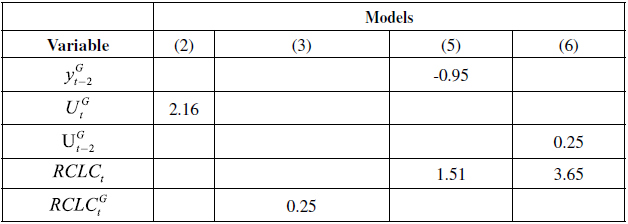
These values confirm the cost in output, unemployment and precariousness (RCLC), which is required to stabilise the economy. Once again, it is clear that the disinflationary adjustment mainly falls on the labour market -to a greater degree than on economic activity- which can be clearly seen in model 6, in which the unemployment gap should widen by 0.25 points to reduce inflation by 1%, at the same time increasing the RCLC by 3.65 percentage points.
CONCLUSIONS AND FURTHER COMMENTS
Between 1970-1982 expansionary fiscal and monetary (populist) policies affected macroeconomic fundamentals, which initiated a long process of high inflation episodes accompanied by drops in output. These stagflation processes were particularly relevant between 1982 and 1988, as a result of which it was called the Lost decade for development. Subsequently, derived from the 1995 financial and macroeconomic crisis (the Tequila crisis), depressions accompanied by inflation were observed again. However, from then on, the independence of the central bank and coherent economic policies caused inflation to decrease progressively. Since the year 2000, it has prevailed at one-digit levels and follows a stationary process. Thus, in contrast with a 52% inflation in 1995, as of 2001 it has remained at levels around 3%, except for the years in which inflation upticks were observed.
In 1998, the Asian and South American turmoils led to a strong inflationary outbreak, as a result of which, since then, we have detected six distinct disinflationary processes, which were addressed by stabilising (contractionary) monetary policy.
The original Phillips Curve (model 58), considering all its modifications and the evolution registered since its release, including its different variants, has been fundamental in the development of macroeconomic theory and economic policy.
The rehabilitation of this curve by the New Keynesian School is crucial in order to comprehend (both the theory and the policy) of the full short -and medium- term macroeconomic equilibrium. Gali and Gertler (1999) conclude that the New Keynesian Phillips Curve provides a good approximation to the dynamics of inflation.
Although the use of this curve in its conventional accelerationist version refers to the output and unemployment gaps, here we added other highly relevant variables of the labour market relative to the rate of critical labour conditions (RCLC). This is done considering that disinflationary costs in Mexico have not been as high as those observed in other countries, when measured exclusively by the increase in the unemployment rate, but when considering the RCLC, the costs have indeed been very high.
Although inflation has not been, at least since 2001, the central problem of the Mexican economy, precariousness conditions, which have characterised the labour market, have been, given that they affect multiple social aspects of a considerable and growing share of the employed population and their dependents. As of the end of 2019, close to 56% of the employed population were informal and over 20% were in critical conditions. Undoubtedly, these marginalising factors have been affecting many aspects of life of the population resulting in social unrest.
In this paper we proved econometrically that, although slack conditions of economic activity and of the labour market explain the disinflationary processes -in line with the main stream theory- since 2005 labour precariousness has been, to a great extent, the escape valve, which has allowed for reducing inflationary pressures, thus stabilising the economy without excessively raising unemployment levels, but rather sharply increasing precariousness.
Labour informality, although significant in a number of models, and contrary to what could be expected, does not seem to have a clear long-term disinflationary effect, which does not mean that it is not a major social and economic concern.
We have shown that since the beginning of the last decade -and perhaps also as an important mechanism of economic re-composition in the wake of the 2009 Great Recession- a combination of phenomena has emerged, which has increasingly affected the quality of employment in Mexico. On the one hand, we have proved that since 2012, when the labour reform was implemented and when the dynamism of economic activity started to diminish, labour precariousness, as it is analysed here, has grown notably.
The profound crisis that the world and Mexico have barely started to witness as a consequence of the Covid-19 pandemic will very likely impact -as never before- the variables that we have analysed here, and they must be the main focus of the forthcoming economic policy, given that they seriously jeopardise the stability of society.
The reported results show that stabilisation and economic and social recovery (Post COVID-19 Society) will not be sustained by unemployment, but by an increasing precariousness in jobs; both those preserved, and those newly generated. We affirm that unemployment will not be the variable that increases substantially as might be suggested by the traditional Phillips curve, but rather, as an extension of our conclusions, it will be the rate of critical conditions that will compensate for the eventual economic recovery. In fact, this is what has been happening since the first variable rose from 2.9% to 3.99% between December 2019 and May 2021; while the rate of critical labour conditions went up from 18.82% to 25.30% of the EAP for the same period, and this trend will likely become even more accentuated in the coming years, which is totally consistent with our main results. Said results are highly alarming in that what has been gained over decades in terms of reducing poverty and inequality will be lost. For these reasons, the issues in question should be central to the economic and policy agenda over the coming years.