Métodos estadísticos para manejar el riesgo de inundaciones y cambio climático

Jery R. Stedinger⁽¹⁾,

(1) Professor of Water Resource Systems Engineering, Cornell University, Ithaca, New York, USA jrs5@cornell.edu

Recibido 23 de octubre de 2012, modificado 1 de noviembre de 2012, aprobado 6 de octubre de 2012

Key words

Flood Frequency Analysis, climate change, stationarity.

Abstract

Actual and potential effects of climate change and climate variability will increasingly challenge hydrologists, civil engineers and planners concerned with flood risk. In general, it is difficult to understand flood risk in particular areas as available records tend to be limited. Our flood quantile estimators are more uncertain than people realize. If we recognize historical climate variability and climate change in our analyses, we will learn that we know even less. In many cases, it is not even clear whether global warming will increase or decrease flood risk. So the challenge is to use all the information available on past floods and future climate, along with a deep understanding of hydrologic processes, to forecast flood risk in the future.

Palabras claves

Análisis de frecuencia de crecientes, cambio climático, estacionariedad

Resumen

El cambio climático real y potencial y la variabilidad del clima se convertirán en un desafío cada vez mayor para los hidrólogos, ingenieros civiles, y planeadores interesados en los riesgos de inundación. En general, no conocemos el riesgo de inundación existente en áreas particulares debido a que los registros tienden a ser limitados. Hay mayor incertidumbre en cuanto a nuestros estimadores cuantiles de inundación –de lo que la gente se imagina–. Si además, para nuestros análisis, tenemos en cuenta la variabilidad climática histórica y el cambio climático, entonces lo que sabemos es aún menos. En muchos casos, ni siquiera está claro si el calentamiento global va a incrementar o a disminuir el riesgo de inundación. Así que el desafío es usar toda la información que tenemos sobre inundaciones pasadas y clima futuro, junto con una profunda comprensión acerca de los procesos hidrológicos, para predecir los riesgos de inundación en el futuro.

INTRODUCTION

Can we predict what changes will occur in the distribution of hydrologic extremes, particularly floods, in a world where we understand that the climate will in fact change? Consider the article "Stationarity Is Dead: Whiter Water Management?" by Milly et al. in [13] The paper generated much excitement in United States and citing it as justification, some people argued that historical records were not going to help us very much because changing climate is a fact. In particular, the paper asserted: "In view of the magnitude and ubiquity of the hydroclimate change apparently now under way, however, we assert that stationary is dead and should no longer serve as a central, default assumption in water-resource risk assessment and planning. Finding a suitable successor is crucial for human adaptation to changing climate".

If we think that hydrology is changing, we then face the challenge of developing a new paradigm for water resource planning. We wrote the paper "From Here to Where?" [19] to address this issue. Does climate change mean that we are not interested in historical records, as some people assert? That, of course, is not true: historical records tell us about floods that occurred in the past, from which we infer the current risk of flooding. we will use this as a starting point and then estimate how and where our journey will take us as things change. And with only modest flood records to define the current risk of flooding, it is difficult to know just where we are headed now. Flood series are highly variable so we understand flood risk with less precision than many people assume.

PRECISION OF FLOOD QUANTILE ESTIMATORS

In [18] and other references provide the standard relationships that describe the precision of flood quantile estimators – but how big are these errors? Beth Faber of the US Army flood engineers generated the example in Figure 1. The flood frequency distribution fit to the Wappinger Creek is the solid line //pink// in the middle of the frequency curves included in the figure. The distributions are displayed on log probability paper, so the reader should be careful when interpreting the results.

In the example, 20-year samples were drawn from the parent distribution (solid line) and were fitted with a 3-parameter log Pearson 3 distribution, as we do in the United States [4] [7], [22]; the distributions shown resulted from that sampling experiment. If one looks at the 1% probability at the bottom corresponding to a return period of 100 years at the top, one sees a range for the 100-year flood running from about 8,000 up to 50,000 cfs: a huge range. Perhaps a 20-year record is too short; so figure 2 provides the corresponding results when one uses 60-year records; now the estimates of the 100-year flood run from 10,000 to 30,000 cfs. Again, that is a wide range.

The examples in Figures 1 and 2 show that we should be modest in our claims of what we understand flood risk to be now. Cohn and Lins in [2] point out that if we incorporate long-term persistence into our analysis, our flood risk estimates appear even less precise. Furthermore, spatial correlation generally decreases the value of regional information [17], [8], [16], [5].

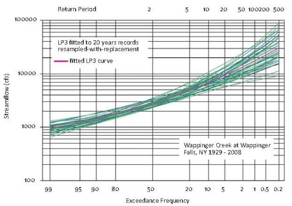
Figure 1. Results of sampling 20-year records from the distribution described by the solid central curve, and fitting a log-Pearson 3 distribution to the data.

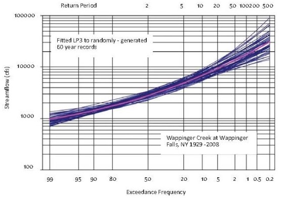
Figure 2. Results of sampling 60-year records from the distribution described by the solid central curve, and fitting a log-Pearson 3 distribution to the data.

CLIMATE SIGNAL IN ANNUAL MAXIMUM FLOOD SERIES

The US. Geological Service put much effort into the question of whether one can see a climate change signal in United States flood records [6] provide a good analysis. They picked 200 of the better stations that should not have been affected by development, and that had 85 - 127 years of record. The paper then regressed the long flow records on annual CO₂ concentration changes over the period of record to see whether there was a statistically significant relationship between flood magnitude and atmospheric CO₂ concentrations. Because individual series only reveal so much, and climate signals should be regional, the United States was divided into four quadrants. A sophisticated block bootstrap/resampling algorithm was employed to see if regional trends were statistically significant.

As shown in Table 1, the only region with strong statistical evidence (significant at the 5% level) of association between floods and global CO₂ is the Southwest (negative). Because the Southwest had the smallest sample size, the chances of a false positive result are largest there. In the Northeast, Northwest, Southeast, and overall for the U.S., there was no discernable signal. Overall in the U.S., as many slopes were positive as were negative, though the Northeast showed more positive trends than negative trends [6]. As in previous studies, on the whole, in the United States we do not see strong and consistent climate-change signals in the frequency of floods. This could be because floods are so variable, or, changes seen in low flows and sometimes mean flows don't manifest themselves in the flood distributions.

Table 1. Hirsch and Ryberg Results on Flood Trends in United States Source: [6]

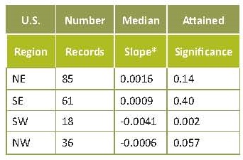
* Percentage change in flood magnitude per 10 ppm increase in CO₂ concentration.

Consider the question: "what should we do differently in terms of flood risk management because of potential climate change?" We do not yet have the ability to document the changes in flood risk in the United States due to greenhouse gas forcing. However, we should maintain an active monitoring strategy so that we can pick up trends as early as possible, by looking where we are most likely to find them: places where modest temperature changes will have important effects. One such place is the Sierra Nevada Mountain, where the snow-line dividing rainfall from snow fall which occurs during any storm can be very sensitive to temperature. As a result, changes in temperature determine, as a function of altitude, whether precipitation rainfall runs off immediately, or is stored as snow and appears later at the outlet of a watershed as snowmelt. And of course, the snow line can move during a storm, rain can fall upon snow resulting in the snow pack storing the rainfall, or rainfall falling on a water-saturated snowpack can result in rapid runoff. Hydrology is an interesting science.

FROZEN BASINS AND CLIMATE CHANGE

Colombia has a glacial zone called the Paramo, which I understand represents 70% of the water supply source for Bogotá; so clearly Colombia has frozen watersheds which are one of the places where climate change is probably first going to be evident, because differences in the partition of precipitation between snow and rain can have major consequences, as does the timing of snowmelt. So will increased temperatures result in larger or smaller flood peaks in glaciated regions?

In [3] report on the impact of increased temperatures in frozen watersheds. One of their concerns is "Does flood risk increase?" Their study considered a subarctic watershed in Sweden where there has been a significant increase in mean air temperature over the past two decades. Thus, they were able to look at historical data and tell us what changes we can see in the hydrology of the area as a result of warmer temperatures. The study considered the 1985- 2009 records for two watersheds: Tarfalajokk that had a 30% glacier cover; and Abiskojokk with a 1% glacier cover. In both watersheds, there was a very clear increasing trend in the mean air temperature; for precipitation there was no change on average, though it seemed to be more highly variable in the latter part of the record. What they found was that in the glacier Tarfalajokk watershed there was a significant increase in the annual floods and the mean summer discharge, so, in fact, floods were greater and flood risk was increased. A smaller glacier resulted in larger flood peaks because the glacier caught less of the summer precipitation. But that was not the case in the Abiskojokk watershed. See Table 2.

Table 2. Observed hydrologic trends in Northern Swedish glaciated and nonglaciated catchments -- analysis of real response to climate warming – 1985 to 2009 Source: [3]

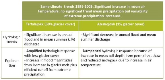
In the Abiskojokk watershed there was a significant decrease in the annual floods and in the mean summer discharge: a completely different hydrological response. The explanation was that in the glacier watershed, the hydrological response was amplified in a large part because there was more base flow from the glacier and the glacier was smaller so more precipitation landed on the ground and ran off. In the unglaciated watershed there is permafrost and the general temperature increase over time reduced the area of permafrost. This resulted in more ground water storage so that rain fall events are partially absorbed. Together these results show that similar climate forcing can cause very different responses in hydrologic systems in the arctic and in the subarctic.

The relationship between precipitation and runoff changed due to a general temperature increase in the region. This is a warning for those who would apply simple rainfall-runoff models to adjusted temperature and precipitation series to explore the likely change in runoff and floods from a watershed. "Permanent" changes such as the depth of permafrost, average soil moisture, or land cover which are not included in such models can be important.

FLOOD RISK AND THE MISSISSIPPI RIVER

So how might we model changes in flood risk and other hydrologic variables. A real but simple study of the Mississippi River provides an illustration. The Mississippi River is one of the largest rivers in the United States.

To illustrate the challenge of forecasting possible climate change, Stedinger and Crainiceanu in [20], [21] used a 1898-1998 record constructed for the Upper Mississippi basin by the US Army Corps of Engineers for their ongoing frequency studies. This data set is different in some aspects from that employed by Olsen et al. in [15], and Matalas and Olsen in [11]. As with the olsen analysis, increasing flood-risk trends were significant in this revised data set using a simple test based on linear regression. While such evaluations have their limitations, the trend at Hannibal, MO, was statistically significant at the 0.01 level using a two-tailed test. This demonstrates that the assumption of independent identically distributed flood peaks can be rejected, and something else seems to be happening.

It could be multi-year persistance, rather than a real trend in [9]. Statistics only tells us that this record is not the result of chance if the annual floods are independent, we do not know if the violation of independence is a trend or some form of multi-year statistical dependence.

To study the impact of different representations of climate variability on flood-risk assessment and project design, we considered three reasonable models: (a) the i.i.d. Log-Normal Model that assumed that the maximum annual floods Q_t are independent, identically distributed random variables where log( Q_t) ∼ N( µ, σ²). This is a traditional model used for flood-risk management. (b) The Log-Normal Trend Model that assumed that the maximum annual floods Q_t have a lognormal distribution around a linear trend, (c) the Log-Normal ARMA Model that assumes that the maximum annual floods Q_t are generated by a stationary low-order Autoregressive Moving-Average (ARMA) process (p, q) for the log-flood series. Parameters of the model are given in Table 3.

Table 3. Parameters of the 3 Models of Annual Flood Maxima for Hannibal (log-space parameters) on the Mississippi. µ is the mean, s the standard deviation of the residuals, b the slope in a linear model for the mean, and the autoregressive term in an ARMA model.

This model explains the observed upward trend as extra variability due to persistence in a stationary time series. The resulting conditional mean for each year of record is shown in Figure 3. The example shows that stationary time-series models are very flexible and produce a reasonable interpretation of historical records that can be used to project flood risk. In this framework, apparent increasing trends in a flood record can be interpreted as the observed parts of a cycle in the natural variation in flood risk. Unfortunately, alternative assumptions and models can lead to very different flood risk forecasts, and it is hard to determine which one is appropriate; it is particularly difficult to distinguish a modest trend from long-term persistence in [5] , which is also likely to be present in [14].

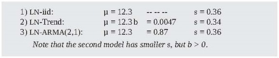
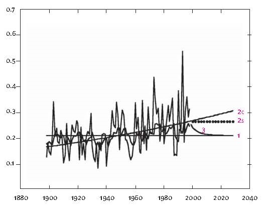
Figure 3. Mean of flood levels over historical record and planning period, for Hannibal record using three flood risk models. (1) LN-iid; (2) LN-Trend, continues [C] or stops [S]; (3) LN-ARMA(2,1) one-step ahead forecast over historical period and forecast for beyond historical record (flood flows in million cfs).w

CONCLUSIONES

The NRC study Decade-to-Century-Scale Climate Variability and Change [14] concludes: "The evidence of natural variation in the climate system -- which was once assumed to be relatively stable -- clearly reveals that climate has changed, is changing, and will continue to do so with or without anthropogenic influences (…) Furthermore, compounding the inevitable hazard of natural climate variations is the potential for long-term anthropogenic climate alteration."

So is stationarity dead? Stationarity remains, in most cases, our paradigm for analyzing historical records. It will be the default for most analyses. One needs to demonstrate that in fact real climate change is affecting the character of the hydrologic series of interest. Stationarity will most likely be the paradigm for analyzing persistence and variability in hydroclimatic records, to which we need to add projected anthropogenic change (which is then a nonstationarity, as were urbanization and development factors in the past).

On the whole, we know the present flood risk at a site with only modest precision because of the limited length of flood records, and the imprecision of regional relationships, assuming annual floods are independent over time. If we allow for historical climate variability, we know even less. In terms of climate change, we need to project from the uncertainty of our current knowledge based upon the past record to estimate the risks in the future. Formulating models is easy, but are they credible? To be defensible, we should base flood-risk forecasts upon some change in climate-characteristics for which we have a physical-causal basis for multi-decadal projections. Global Circulation Models (GCMs) have been employed to provide a linkage between the global release of greenhouse gases and local watershed hydrology, but whether they are up to the task is highly questionable in that those global models fail to adequately represent thehydrologic process on a watershed scale [1], [12], [10]. And even if climate has been stationary, for at least a century man has been changing and will continue to change the landscape and hydrologic systems across the United States as well as most other parts of the world. Change in flood risk is not new.

FOOTNOTES

*Este artículo es el resultado de la ponencia de Jery R. Stedinger presentada en el foro "Hidrología de extremos y cambio climático que se llevó a cabo en la Universidad de los Andes el día 28 de junio de 2012.

REFERENCES

[1] V.K. Arora. "Streamflow simulations for continental-scale river basins in a global atmospheric general circulation model", Adv. in Water Resources 24, 775-791, 2001.         [ Links ]

[2] T. A. Cohn, and H. F. Lins. "Nature’s style: Naturally trendy". Geophysical Research Letters, Vol. 32, No. 23402, December, 2005, pp 1-5        [ Links ]

[3] H.E. Dahlke, S.W. Lyon, J.R. Stedinger, G. Rosqvist and P. Jansson. "Contrasting trends in floods for two sub–arctic catchments in northern Sweden – Does glacier presence matter ?" Presented in: Hydrol. Earth Syst. Sci. , [electronic medium] Available www.hydrol-earth-syst-sci.net/16/2123/2012/, 2012.         [ Links ]

[4] V.W. Griffis, and J. R. Stedinger. "Evolution of Flood Frequency Analysis with Bulletin 17". J. of Hydrol. Engineering, Vol., 12 No. 3, February 2007, pp. 283-97.         [ Links ]

[5] A.M. Gruber, J.R. Stedinger, Models of LP3 Regional Skew, "Data Selection, and Bayesian GLS Regression". In World Environmental & Water Resources Conference 2008 AHUPUA'A, paper 596, R. Babcock and R. Walton (eds.), Hawaii, Amer. Soc. of Civil Engineers, May, 2008.         [ Links ]

[6] R.M. Hirsch, and K. R. Ryberg. "Has the magnitude of floods across the USA changed with global CO2 levels?" Hydrological Sciences Journal, Vol.,57 No. 1, October, 2011, pp 1-9.         [ Links ]

[7] Interagency Committee on Water Data (IACWD), Guidelines for determining flood flow frequency: Bulletin 17B (revised and corrected), Washington D.C: Hydrol. Subcomm, 1982, pp. 28        [ Links ]

[8] M. Jin and J.R. Stedinger, "Flood Frequency Analysis with Regional and Historical Information" Water Resources Research, Vol., 25 No.5, December, 1989, pp.925-936,         [ Links ].

[9] Kiem, A. S., S. W. Franks, and G. Kuczera, "Multi-decadal variability of flood risk". Geophysical Res. Letters, Vol., 30, No. 2, January 2003, pp.1-4        [ Links ]

[10] Z. W.Kundzewiczab, and E. Z. Stakhiv, "Are climate models "ready for prime time" in water resources management applications, or is more research needed?" Hydrological Sciences Journal, Vol., 55 No.7 October, 2010, pp.1085-1089        [ Links ]

[11] N.C. Matalas, and J.R. Olsen. "Analysis of trends and persistence in hydrologic records, Risk-Based Decision Making in Water Resources IX" in Proceedings of the Ninth Conference, United Engineering Foundation, Santa Barbara, CA: Amer. Society of Civil Engineers, October, 2001. pp. 61-76.         [ Links ]

[12] P. C. Milly, D. J. Betancourt, M. Falkenmark, R.M. Hirsch, Z.W. Kundzewicz, D.P. Lettenmaier, and R.J. Stouffer, "Stationarity is dead: Whither water management". Science. Vol., 319, No. 5853. February, 2008, pp. 573-574.         [ Links ]

[13] P. C. Milly, K. A. Dunne1 & A. V. Vecchia. "Comparison of streamflow: 1900-1970 to 1971-1998" Nature, Vol., 438 No. 17, 2005, pp. 347- 350.         [ Links ]

[14] National Resources Council, Decade-to-Century-Scale Climate Variability and Change: A Science Strategy, Panel on Climate Variability on Decade-to-Century Time Scales, Washington, D.C: National Academy Press, 1998.         [ Links ]

[15] J.R Olsen, J.R Stedinger, N.C. Matalas, and E.Z. Stakhiv, "Climate variability and flood frequency estimation for the Upper Mississippi and Lower Missouri Rivers" J. of the Amer. Water Resources Association, Vol., 35 No. 6, December 1999, pp.1509-1524,         [ Links ]

[16] D. S. Reis, J. R. Stedinger, and E. S. Martins. "Bayesian generalized least squares regression with application to log Pearson type 3 regional skew estimation" Water Resource. Vo., 41, W10419, 2005, pp. 1-14         [ Links ]

[17] J.R. Stedinger, and G.D. Tasker. "Regional Hydrologic Analysis 1. Ordinary, Weighted and Generalized Least Squares Compared" Water Resources Research, Vol., 21 No. 9, June 1985, pp.1421-1432.         [ Links ]

[18] J.R. Stedinger, R.M. Vogel and E. Foufoula-Georgiou. "Frequency Analysis of Extreme Events Chapter 18", in Handbook of Hydrology, D. Maidment (ed.), New York: McGraw-Hill, 1993, pp. 18-26        [ Links ]

[19] J.R. Stedinger, and V.W. Griffis. "Getting From Here to Where? Flood Frequency Analysis and Climate" J. Amer. Water. Resour. Assoc., Vol., 47 No.3, June 2011, pp. 506-513        [ Links ]

[20] J.R., Stedinger and C. M. Crainiceanu. "Climate Variability and Risk Forecasting" in Proceedings 2002 Conference on Water Resources Planning and Management, Edited by D.F. Kibler, paper D-7-329, Virginia: Amer. Society of Civil Engineers, Reston, 2002.         [ Links ]

[21] J.R, Stedinger, and C. M. Crainiceanu, "Climate Variability and Flood-Risk Management", in Risk-Based Decision Making in Water Resources IX, Proceedings of the Ninth Conference, United Engineering Foundation , Santa Barbara, CA,: Amer. Society of Civil Engineers, Reston, 2001 pp. 77-86        [ Links ]

[22] J.R. Stedinger, and V.W. Griffis, "Flood Frequency Analysis in the United States: Time to Update" J. of Hydrology, Vol., 13 No. (4), April 2008, pp.199-204.         [ Links ]