CFD modeling of Air-Water Two-phase Annular Flow before a 90° elbow

Modelamiento en CFD de flujo anular bifásico aire-agua en una tubería antes de un codo de 90°

Andrés Felipe Melo Zambrano ⁽¹⁾, Nicolas Ratkovich ⁽²⁾

⁽¹⁾B.S. in Chemical Engineering, University of Los Andes. Bogotá, Colombia. af.melo730@uniandes.edu.co

⁽²⁾ Ph.D, MSc., Assistant Professor, University of Los Andes, Department of Chemical Engineering, Product and Process Design Group (GDPP). Bogotá, Colombia. nrios262@uniandes.edu.co

Received August 4^th, 2015. Modified November 16^th, 2015. Approved November 20^th, 2015.

DOI:http//:dx.doi.org/10.16924/riua.v0i43.843

Key words

Annular Flow, CFD, Two-Phase Flow, Water-Air System.

Abstract

In this work, a Computational Fluid Dynamics model is presented for the analysis of annular air-water flow before a 90° bend with a radius to diameter ratio (r/D) of 1.5, implementing the Volume of Fluid (VOF) model in STAR-CCM+ v9.2. An 8m-long vertical tube with an internal diameter of 0.076 m was studied for ten different air and water superficial velocities. The mean void fraction was compared between the experimental measurements, the CFD model, and a model in OLGA. The CFD and OLGA model presented an average relative error of 8.79 % and 17.05 %, respectively.

Palabras clave

CFD, flujo anular, flujo bifásico, sistema aire-agua.

Resumen

En este trabajo se presenta un modelo en Dinámica Computacional de Fluidos (CFD) para el análisis de flujo anular bifásico agua-aire antes de un codo de 90°, implementando el modelo de Volumen de Fluido (VOF) en STAR-CCM+ v9.2. Se analizó una tubería de 8 m de largo y un diámetro interno de 0.076 m, evaluando 10 condiciones experimentales de velocidad superficial de aire y agua. La fracción de vacío promedio se comparó para los resultados experimentales contra un modelo en CFD y en OLGA, los cuales presentaron un error relativo medio de 8.79% y 17.05%, respectivamente.

Introduction

The chemical, O&G, and nuclear industries, frequently involve the transportation of single and multiphase flows. In some applications such as feeding raw material to a process, recovering products or residuals, and recirculating cooling or heating fluids, the transport is mainly a single phase flow, involving less severe problems than multiphase flows. Within the O&G industry, two-phase flows are encountered such as oil-gas or oil-water systems, and three-phase flow, oil-gas-water. Furthermore, pipeline systems are used between offshore platforms and onshore installations for oil and gas transportation. Most pipeline systems include accessories either for redirecting fluids, mixing two different fluids, or for flow control. Although, these accessories contribute to a more dynamic and flexible design, they generate changes in flow patterns, larger pressure drops, and cause problems such as erosion and partial or total failures in pipelines downstream (Mazumder, 2012b). The study of multiphase flows is, therefore, of great interest when it comes to attempting to avoid financial costs associated with pipeline maintenance and repair (Abdulkadir, 2011).

In two-phase liquid-gas flow, phases can be distributed in different ways known as flow patterns. It is important to identify the flow pattern, since significant parameters such as liquid hold-up and pressure drop depend on it. In horizontal flow, the gravity force acts perpendicular to axial direction, which may result in phase separation. The main flow patterns in horizontal flow are: bubbly, stratified, slug and annular flow. In bubbly flow, the gas phase is distributed in the form of dispersed bubbles in the continuous liquid phase. In a stratified flow, there is a smooth liquid-gas interface, without droplet entrainment in the gas phase, which travels above the liquid phase (Crowe, 2005). Slug flow is characterized by the presence of bullet-shaped bubbles, called Taylor bubbles that travel on the top of the pipe, and the continuous liquid phase exists in the form of liquid slugs. In annular flow, the gas phase travels in the center of the pipe, while the liquid phase appears in the form of a thin liquid film around the gas core. For vertical pipes, the flow patterns are: bubbly, slug, churn, and annular flow. Churn flow is considered a transition regime between slug and annular flow.

The above sheds light on the importance of a detailed study of the behavior of such types of flow. Since conducting experiments using oil-gas is quite expensive, low-cost fluids with similar properties are used so that experimentation is easily replicable. Computational Fluid Dynamics (CFD) models are complementary tools for the experiments. The main advantages of these models are lower associated costs, fewer limitations in complex studies, higher replicability, and the required time to design and develop the studied cases (Abdulkadir, 2011). In order to develop CFD models capable of predicting multiphase flow, it is necessary to validate models for simple systems by means of experimental results. Thus, it is possible to change the fluid properties, for instance viscosity and density, with properties of more challenging systems, for instance, oil-gas.

Different experimental researches for air-water two-phase flow in a 90° bend have been carried out to measure different flow properties and system conditions, and compared with empirical correlations (Silberman, 1960; Kim et al., 2006; Benbella et al., 2008; Silva et al., 2010). CFD models have only been developed over recent years and to a lesser extent than experimental studies, and they are usually compared with empirical correlations and experimental research (Mazumder et al., 2011; Mazumder, 2012a; Mazumder, 2012b).

Materials and Methods

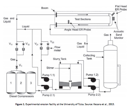
The Department of Mechanical Engineering at the University of Tulsa, OK (USA) has an experimental facility (Fig. 1), in which erosion experiments are performed. The main equipment used includes: a compressor, slurry tank, a liquid and gas injector, a trial section and a storage tank. In addition, the test section has a length of 18m and can use two different diameters. The detailed experimental set-up is reported by Kesana et al. (2013).

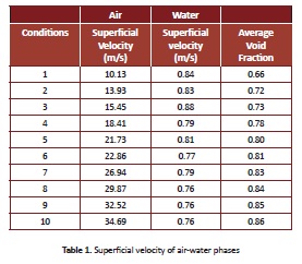
The experiments (Table 1) were performed with using standard absolute viscosities and densities for air,of 0.01 cP and 1.23kg/m³ for air,, and of water, 1 cP and 998.00kg/m³for water, respectively. A surface tension, temperature, and pressure of 0.74 N/m, 298 K and 101325 Pa were used, respectively. The experiment was conducted for a total time of 60 s and the data was reported with a frequency of 10,000 Hz.

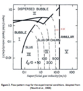
As a first approximation to the experimental conditions, a flow-pattern map was used (Fig. 2). Although, this map was developed for pipe diameters of 0.051m, the transition to annular flow is independent of the diameter. Therefore, this map may be used for a pipe diameter of 0.076 m for this case. According to the map, the first two conditions correspond to transition or slug flow, and annular flow for the remaining conditions, due to the high and low superficial gas and liquid velocities, respectively.

CFD model

The CFD methodology consists of three different stages. In the first stage, pre-processing, the geometry and mesh are generated, initial and boundary conditions are defined, and the physical models are selected. In the second stage, the solution models are prescribed, and the last stage corresponds to the results obtained from the simulation.

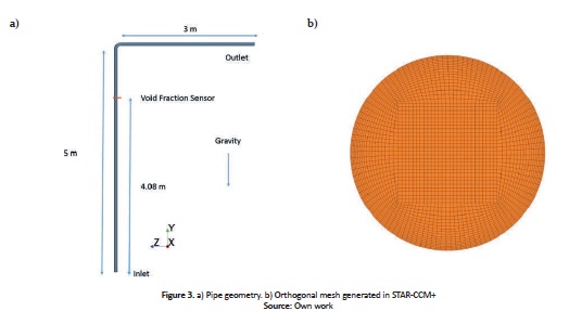
A 3D pipe was built in STAR-CCM+ v9.2 (Fig. 3a), in which the vertical and horizontal sections were 5m and 3m long, respectively. The 90° bend had a radius of curvature of 0.114m (D/L =1.5) and the tube, a diameter of 0.076m. A butterfly mesh (Fig. 3b) was used for all conditions, which has been proved to be the most accurate type when modeling two-phase flows, according to the study by (Hernandez et al., 2010), and has been used successfully by (Hernandez, 2007; Tkaczyk, 2011; Abdulkadir et al., 2013) for two-phase flow CFD modeling. In order to correctly capture the interface between both phases, a fine grid quality close to the wall is required. Therefore, 18 layers near the pipe wall were used and the mesh was generated using the directed meshing operation in STAR-CCM+. In order to verify mesh independency for the solution, a grid independency test was performed based on the factors h_normal/h_fine and h_coarse/h_normal equal to 1.3, where h is th e cell length, as suggested by (Celik et al., 2008).

The problem addressed in this paper consists in the study of two-phase flow dynamics, for which Navier-Stokes equations were used as the main tool. In STAR-CCM+ transport equations were solved in their integral form using the finite volume method. The Volume of Fluid Model (VOF) is based on the spatial distribution of each phase inside the pipe in a specific period of time-the void fraction-and the interface between both phases is solved with the surface tension, which acts as a body force. The VOF model assumes that all phases share the same fields for the variables and properties, solving only a set of equations for fluid transport. In addition, the VOF model considers a conservation equation for the void fraction of the mixture.

As a result of the unsteady behavior of the flow pattern and the properties of mixture given by the VOF model, the Reynolds-averaged Navier-Stokes equations were used. Therefore, in order to simulate a turbulent flow, a turbulence model has to be used. The k-ω model consists of two transport equations, the first for k, the turbulent kinetic energy, and the second equation for ω, the specific rate of dissipation; these are required as closure for the RANS equations. The advantages of using this model are an improved performance for the boundary layer and the fact that it can be applied in the region dominated by viscous forces. On the other hand, the main drawback of this model is its significant sensitivity to the boundary conditions at the entrance (CD-Adapco, 2014). Considering the performance of the k-ω model for the boundary layer and the main characteristics of anular flow, this model was used instead of the k-ε.

The implicit model is used for the temporal discretization of the Navier-Stokes equations when studying turbulent flows. The time step ∆t, directly affects the solution and convergence of the simulation. It has to maintain the convective Courant number between 0.25 and 1, to ensure that a fluid particle moves one cell in one time-step. The time step was calculated with a Courant Number equal to 1.

The inlet was defined as inlet velocity, and the outlet as pressure outlet. The velocity was prescribed as the sum of the superficial velocities of both phases, whereas the void fraction was prescribed as a homogenous mixture, defining one half of the inlet as the liquid phase and the other as the gas phase. The domain of the pipe was initialized only with water. At the pipe wall, the no slip condition was assumed, due to the fact that the fluid in contact with the wall is stationary. In order to obtain a mean void fraction, a surface average monitor was located at 0.91m before the inlet of the 90° bend.

OLGA (OiL and GAs) model

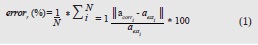
A comparison between the experimental data and a model in OLGA v7.3 was performed. The OLGA model uses the point model, which assumes a steady state and a fully developed flow (Schlumberger, 2014). The absolute average relative error-Eq. (1)-was calculated for this comparison between the experimental and OLGA void fraction.

α_corri is the void fraction obtained for each CFD or OLGA result. α_expi is the ith data of void fraction for experimental results. N is the total number of data taken into account for the error calculation.

Results and discussion

The void fraction was calculated for the grid independency test as the void fraction average in the last second of the simulation, and the simulation error (Table 2) was calculated as the absolute average relative error between the experimental and simulation void fraction.

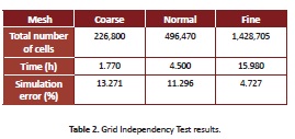
As expected, the lowest error corresponds to the result obtained by the fine mesh, due to the fact that the cells have a smaller volume compared to the other cases. On the other hand, the error using the coarse mesh was lower than with the normal mesh due to the uniformity of the cells, with a ratio of 0.13 and 0.15 respectively. The uniformity of the cells was calculated as the ratio between the length of the horizontal and vertical sides of the cell.

Comparison with OLGA model

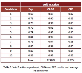
Comparing the experimental results with the OLGA model, an error of 17.05% was obtained (Table 3). It must be considered that this software cannot define an accessory such as a 90° bend. In addition, OLGA was designed for large-scale studies, which can lead to errors when working with small diameter pipes. Also, OLGA identified the flow pattern for the ten conditions as slug flow. This result is in accordance with the identified flow patterns for the first two conditions, using the flow-pattern map. Given that the software assumes a stationary model, it may not be able to capture the transition between slug and annular flow for the other conditions.

CFD Simulation

The residuals of the equations solved by STAR-CCM+ clearly showed that the residuals of the solved equations are stable as from 5,000 iterations or 0.25s, until the end of the simulation. Therefore, the simulation converged properly for all studied conditions. These results were obtained using a physical time of 5s and a cluster with 55 cores.

For all conditions, an error of 8.79 % was found (Table 3) by comparing the experimental and CFD average void fraction at the last second, using Eq. (1). Analyzing the CFD results, the error obtained for all conditions is relatively low. This may be due to the fact that the VOF model used in this study uses only one momentum equation for both liquid and gas phases. Since the superficial velocities are considerably different, the VOF model could present a limitation in this case. Despite this, one can conclude that the model is able to predict the average void fraction relatively well.

Phase distribution

The phase distribution inside the pipe for the experimental and simulation sensors are presented in Fig. 4 for conditions 1 and 8.

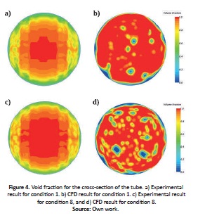
For the first condition, comparing CFD results with the experimental data, the following was found: (i) areas in the center of the pipe in the CFD results show that droplets are present in the gas phase indicating annular flow, or that this phase is sufficiently unstable and liquid slugs can break showing a a characteristic of transition flow. (ii) The experimental results show that the gas phase is concentrated in the center of the tube and the liquid film is concentrated near the pipe wall, which may indicate that the Taylor bubble travels down the center, characterizing a slug or transition flow. (iii) For condition 8, it can be clearly observed that the liquid film is significantly thinner compared to the first condition, because superficial gas velocity is higher, for both experimental and CFD results. A transition flow may be identified, but with a more annular behavior in contrast to the first condition.

The differences between experimental and CFD phase distributions are significant due to the limitation of the VOF model, given that the superficial velocities are considerably different. Using a finer mesh near the center of the pipe or the same frequency in the experimental measurements and the CFD model, the latter could capture the liquid slugs that are clearly observed in the experimental cross section.

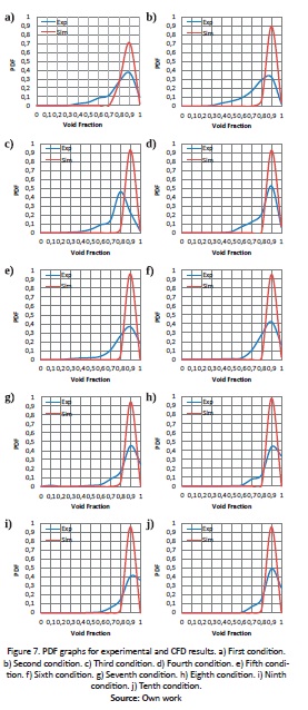
Probability Density Function (PDF)

The probability density function (PDF) was used (Fig. 5) in order to analyze the flow pattern for conditions 1 and 8. Comparing experimental and CFD results, the following was found: (i) experimental results for both conditions show only one peak with a probability of less than 0.5, and a significant left tail. (ii) Both CFD results clearly show a defined peak at 0.9 and a probability equal to or greater than 0.7, with more annular behavior than the experimental data. (iii) A transition flow for both conditions and results can be identified, due to the shape of the graph, according to Costigan et al. (1997). It is important to highlight that in the study reported by Costigan et al. (1997) a different pipe diameter was used.

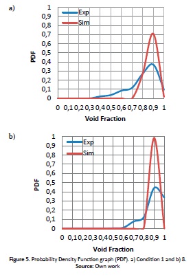
The significant differences between both probability density function graphs, may be a result of the different frequencies used in the experimental measurements and CFD model, 10,000 HZ and 2,000 Hz respectively, and the VOF limitations mentioned above.

Conclusions

A CFD analysis was performed with STAR-CCM+, for air-water two-phase flow in a 90° bend with a pipe diameter of 0.76 mm. An absolute average relative error of 8.79% was found using a butterfly mesh of 1,428,705 cells and a physical time of 48h approximately for each simulation. Considering the VOF model only uses one momentum equation for both phases, the CFD model presented good agreement with the experimental data.

The OLGA model reported a significantly high error of 17.05 % compared to CFD. This difference is mainly due to the fact that the point model used in OLGA assumes a steady state and that the software is designed for large-scale studies. Therefore, the model will not be able to capture the oscillation presented in the void fraction measurements due to the liquid slugs, that is, the flow pattern, and its extension to short pipe lengths and accessories may result in significant errors.

The analysis performed of the flow pattern with phase distribution is not sufficient to reach any accurate conclusions. Possibly, by using a finer mesh or a different model from the VOF, the CFD model could capture the liquid slugs that are observed in the experimental results and a better analysis could be performed. This behavior may be caused by the difference between the frequency for the experimental measurements and the CFD model, 10,000 Hz and 2,000 Hz, respectively. The PDF graphs showed a considerable difference between the experimental and simulation results. Since the superficial gas velocities are significantly higher than the liquid velocities, the VOF model may not be able to correctly capture the liquid slugs presented in the experimental results.

Acknowledgments

The authors acknowledge Dr. Mazdak Parsi for providing the experimental data from the University of Tulsa. The authors gratefully acknowledge Schlumberger for providing the OLGA software as well as Universidad de los Andes for their support in this project. Finally, the authors want to acknowledge Prof. Rodrigo Marin (Universidad de los Andes) for his continual assistance with the Schlumberger software.

References

Abdulkadir M, Hernandez-Perez V, Lo S, Lowndes I S and Azzopardi B J. (2013). Comparison of Experimental and Computational Fluid Dynamics Studies of Slug Flow in a Vertical 90 ° Bend. The Journal of Computational Multiphase Flows, 5(4), 265-284. DOI: 10.1260/1757-482X.5.4.265.         [ Links ]

Abdulkadir M. (2011). Experimental and Computational Fluid Dynamics (CFD) Studies of Gas-Liquid Flow in Bends. University of Nottingham, 384.         [ Links ]

Benbella S, Al-Shannag M & Al-Anber Z. (2008). Gas-Liquid pressure drop in vertical internally wavy 90° bend. Experimental Thermal and Fluid Science, 33(2), 340-347. doi:10.1016/j.expthermflusci.2008.10.004.         [ Links ]

Bratland O. (2010). Pipe Flow 2 Multi-phase Flow Assurance.         [ Links ]

CD-Adapaco. (2014, 11 20). STAR CCM+ Documentation. 2014.         [ Links ]

Celik I., Ghia U, Roache P., Freitas C., Coleman H. & Rand P. (2008). Procedure for Estimation and Reporting of Uncertainty Due to Discretization in CFD Applications. Journal of Fluids Engineering, 130(7). doi:10.1115/1.2960953.         [ Links ]

Costigan G. & Whalley P. B. (1997). Slug flow regime identification from dynamic void fraction measurements in vertical air-water flows. International Journal of Multiphase Flow, 23(2), 263-282. doi:10.1016/S0301-9322(96)00050-X.         [ Links ]

Crowe C. T. (2005). Multiphase Flow Handbook. New York: Taylor & Francis Group.         [ Links ]

Hernandez V, Abdulkadir M. & Azzopardi B. J. (2010). Grid Generation Issues in the CFD Modelling of Two-Phase Flow in a Pipe. Journal of Computational Multiphase Flows, 3 (1). doi: http://dx.doi.org/10.1260/1757-482X.3.1.13.         [ Links ]

Hernandez V. (2007). Gas-Liquid two-phase flow in inclined pipes. University of Nottingham, 294.         [ Links ]

Hewitt F., Delhaye M. & Zuber N. (1986). Multiphase Science and Technology. Berlin: Springer-Verlag.         [ Links ]

Kesana N. R., Grubb S. A., McLaury B. S. & Shirazi S. A. (2013). Ultrasonic Measurement of Multiphase Flow Erosion Patterns in a Standard Elbow. Journal of Energy Resources Technology, 135(3). doi: 10.1115/1.4023331.         [ Links ]

Kim S. (2006). Two-Phase Frictional Pressure Loss in Horizontal Bubbly Flow with 90-Degree Bend. ASME, 7.         [ Links ]

Mazumder Q. H. & Siddique S. (2011). CFD Analysis of Two-Phase Flow Characteristics in a 90 Degree Elbow. Journal of Computational Multiphase Flow, 3(3).         [ Links ]

Mazumder Q. H. (2012). CFD Analysis of Single and Multiphase Flow Characteristics in Elbow. Scientific Research Publishing, 4(4). doi: 10.4236/eng.2012.44028.         [ Links ]

Mazumder Q. H. (2012). CFD Analysis of the Effect of Elbow Radius on Pressure Drop in Multiphase Flow. Modelling and Simulation in Engineering, 2012. doi: 10.1155/2012/125405.         [ Links ]

Schlumberger. (2014, 11 19). OLGA Documentation. 2014.         [ Links ]

Silberman E. (1960). Air-Water Mixture Flow through Orifices, Bends, and other Fittings in a Horizontal Pipe. University of Minnesota.         [ Links ]

Silva S., Luna J. C., Carvajal I. & Tolentino R. (2010). Pressure Drop Models Evaluation for Two-Phase Flow in 90 Degree Horizontal Flows. Sociedad Mexicana de Ingeniería Mecánica, 3(4).         [ Links ]

Tkaczyk P. (2011). CFD simulation of annular flows through bends. University of Nottingham, 185.         [ Links ]

Appendix

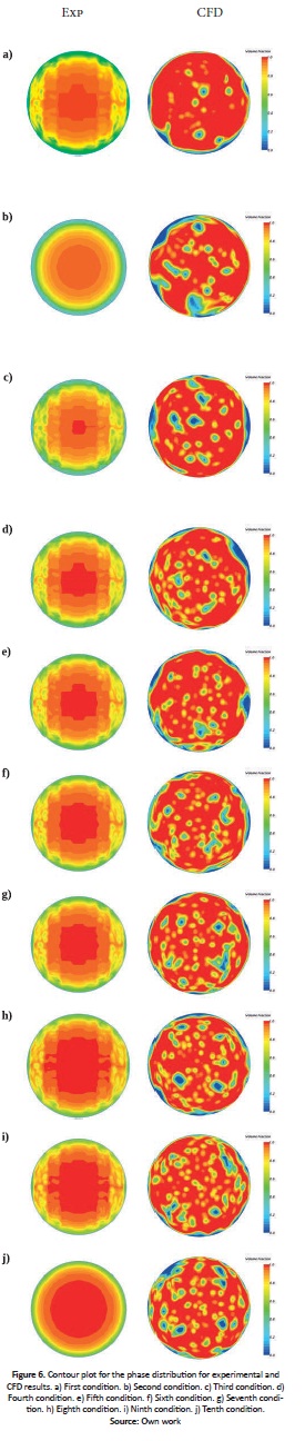
Appendix A. Contour of the phase distribution

Fig. 6 illustrates the contour of the void fraction for the experimental and CFD results for all ten conditions.

Appendix B Probability density function graphs

Fig. 7 shows the PDF graphs for the experimental and CFD results for all ten conditions.