James W. Kolari* & Ignacio Vélez-Pareja^**

* PhD Arizona State University. MBA Western Illinois University. JP Morgan Chase Professor of Finance Texas A&M. Correo electrónico: j.kolari@tamu.edu

^** M.Sc. En ingeniería industrial University of missouri Columbia, missouri, Usa. ingeniero industrial, Universidad de los andes, Bogotá, Colombia Profesor de tiempo completo Universidad tecnológica de Bolívar, Cartagena, Colombia. Correo electrónico: nachovelez@gmail.com

Recibido: noviembre de 2011 Aceptado: septiembre de 2012

Abstract:

The value of debt tax shields in foundational corporate valuation models by nobel laureates modigliani and Miller (MM) continues to be a controversial issue that is central to our understanding of corporate finance. Rather than discounting debt interest payments using a riskless interest rate or unlevered equity rate, the present paper proposes the use of the levered cost of equity. Assuming no bankruptcy risk and no personal taxes, our revised tax model yields an inverted U-shaped firm value function with an interior optimal capital structure. Analyses are extended to Miller's personal tax extension of MM's tax model. Also, implications to corporate capital structure decisions and previous literature are discussed.

Keywords: value of tax shields; Capital structure; Firm valuation; share valuation

Resumen:

El valor del ahorro de impuestos de la deuda en los modelos fundamentales de valoración de empresas de los Premios nobel modigliani y Miller (MM) continúa siendo un tema controversial que es fundamental para nuestra comprensión de las finanzas corporativas. En lugar de descontar los pagos de intereses de la deuda con una tasa de interés libre de riesgo o la tasa del patrimonio sin apalancamiento, el presente trabajo propone el uso del costo del patrimonio con deuda. Suponiendo que no hay riesgos de quiebra y no hay impuestos personales de renta, nuestro modelo de impuestos una vez revisado obtiene una función del valor de la firma en forma de U invertida con una estructura óptima de capital interior. Los análisis se extienden a la extensión Miller con impuestos personales para el modelo con impuestos de MM. Además, se discuten la literatura existente y las implicaciones para las decisiones empresariales de estructura de capital.

Palabras clave: valor del ahorro de impuestos, estructura de capital, valoración de empresas, la valoración de acciones.

Résumé :

La valeur de l'épargne d'impôts de la dette dans les modèles fondamentaux d'évaluation des entreprises des prix Nobel Modigliani et Miller (MM) continue à être un thème controversé qui est fondamental pour notre compréhension des finances corporatives. Au lieu de décompter les paiements d'intérêts de la dette avec un taux d'intérêt libre de risque ou le taux de patrimoine sans effet levier, ce travail propose l'utilisation du coût du patrimoine avec la dette. Supposant l'inexistence de risques de faillite et d'impôts personnels de rente, notre modèle d'impôts obtient, après révision, une fonction de la valeur de la firme en forme de U inverti avec une structure optimum de capital intérieur. Les analyses s'étendent à l'extension Miller avec des impôts personnels pour le modèle avec impôts de MM. La littérature existante est également discutée ainsi que les implications pour les décisions entrepreneuriales de structure de capital.

Mots-Clefs : Valeur de l'épargne d'impôts, Structure de capital, Évaluation d'entreprises, Évaluation d'actions

Resumo:

O valor da economia de impostos da dívida nos modelos fundamentais de valoração de empresas dos Prêmios nobel modigliani y Miller (MM) continua sendo um tema controvertido e fundamental para nossa compreensão das finanças corporativas. Em vez de descontar os paga-mentos de juros da dívida com uma taxa de juro livre de risco ou com a taxa do patrimônio sem influência , o presente trabalho propõe o uso do custo do patrimônio com dívida. Supondo que não há riscos de quebra e não há impostos pessoais de renda, nosso modelo de impostos depois de revisado obtém uma função do valor da firma em forma de U invertida
com uma ótima estrutura de capital interior. As análises se estendem à extensão Miller com impostos pessoais para o modelo com impostos de MM . Além disso, discutem-se a literatura existente e as implicações para as decisões empresariais de estrutura de capital.

Palavras-chave: valor da economia de impostos, estrutura de capital, valoração de empresas, valoração de ações.

Corporate valuation theories by nobel laureates modigliani and Miller (hereafter MM) (1958, 1963) have become cornerstones of modern thinking about capital structure. Relevant to real world practice, their debt tax gain arguments would tend to favor the use of financial leverage by firms and individuals in capital markets. In view of recent leverage excesses that contributed to the financial and economic crises of 2008 and 2009, after more than 50 years of debate and extensive empirical evidence,² it would seem worthwhile to revisit the long-standing controversy surrounding MM's tax valuation model. The main dispute focuses on how to compute the present value of interest tax deductions on debt. Initiating the debate, in their original tax model in 1958, MM used the unlevered equity rate to discount interest tax deductions and proposed relatively modest tax gains on debt interest; however, in 1963 MM overturned their earlier original tax model and proposed a tax correction model that discounted interest tax deductions at the riskless debt rate to yield very large debt tax gains.

Motivated by excessively large debt tax shields that did not coincide with observed corporate practice, Miller (1977) extended MM's tax correction valuation model to personal taxes and proposed that interest tax gains on debt have little or no value for most firms. Excluding personal taxes, some authors subsequently returned to MM's original tax model approach by discounting interest tax deductions at the unlevered equity discount rate, including Harris and Pringle (1985), Modigliani (1988), and Kaplan and Ruback (1995). Also, Miles and Ezzell (1980, 1985) and Arzac and Glosten (2005) proposed to discount tax shields at the riskless rate in the first period but at the unlevered equity rate thereafter. Consistent with these studies, Grinblatt and liu (2008) viewed the debt tax shield as a derivative of the underlying unlevered asset (and its cash flows) and used option pricing methods to derive its value. Other researchers have employed the cost of risky debt to discount interest tax deductions, such as myers (1974), Luehrman (1997), Damodaran (2006), and others, which assumes that the only risk associated with interest tax deductions (i.e., tax shields) is the risk of debt. Given risky debt in which earnings before interest and taxes may possibly be less than interest, Wrightsman (1978) argued that the tax shield would be reduced compared to using the riskless rate because the effective tax shield from debt will depend on operating earnings. In general, these alternative discounting approaches³ tend to diminish the present value of tax gains on debt and thereby soften MM's 1963 conclusions.

More recently, Ross (2005) has commented that MM's static tax correction model is flawed. In his words, "a flaw in the traditional approach occurs [...] by valuing the cash flow of the tax shield at the riskless debt rate. [...] as Miller (1977) argues, the tax shield goes to the equity holders and not the bondholders and the discount rate at which it should be valued should depend on the marginal tax rate of equity holders and not debt holders." (2005, p. 7) since debt tax gains are passed to shareholders as dividends,⁴ he applied the personal equity tax rate to the tax shield.

Defining after-tax equity value with interest tax deductions as the sum of the after-tax equity value with no interest deductions plus the tax gain from interest deductions, which is consistent with MM's tax models (i.e., all tax gains are paid out to shareholders), it is shown that the after-tax value of equity with no interest deductions becomes negative when debt values exceed the unlevered value of the firm. Due to limited liability and no bankruptcy risk, equity value with or without interest deductions cannot be negative. This unreasonable result occurs even with no bankruptcy risk when discounting interest tax shields using both risky debt rates and unlevered equity rates in their tax models.⁵ to overcome this problem, a revised tax model is proposed which that discounts interest deductions using the levered cost of equity. This approach provides a robust tax valuation paradigm within MM's framework that gives positive equity values with and without debt tax gains. To the authors' knowledge, no previous papers have investigated this logically appealing levered equity rate discounting approach within the MM tax model framework. Upon doing so, the valuation results help mitigate a number of criticisms of MM's tax models, contribute to reconciling theory and evidence on capital structure and firm valuation, and provide new insights into the role of debt tax shields in firm valuation.

Section 1 briefly overviews MM's original and tax correction valuation models. Section 2 applies a portfolio approach to compare equity valuation results using different discount rates to find the present values of interest deductions. Section 3 provides numerical examples that show the proposed revised tax model using the cost of equity to discount interest deductions overcomes negative equity and related negative cost of equity problems. Following Miller (1977), section 4 extends the analyses to personal taxes, which shows that, unlike MM's tax correction model, the revised tax model is little changed and therefore robust to personal taxes. Section 5 discusses implications to corporate capital structure decisions and related literature that bode well for the revised tax model's valuation of debt tax shields. Section 6 concludes.

According to Proposition I of Modigliani and Miller's (MM) (1958) original valuation model without corporate taxes (but no personal taxes), firm valuation is independent of capital structure. However, taxes result in a tax gain on debt interest deductions. In MM (1958) the unlevered equity rate is used to discount debt interest deductions but in MM (1963) the much lower riskless debt rate is used for discounting purposes, which resulted in a large tax gain on debt usage to the firm and its shareholders. In the absence of bankruptcy risk, Proposition I was soundly rejected in favor of an extreme all-debt capital structure corner solution. In a 1988 rejoinder to the MM tax correction paper, Miller (1988) commented that: "We must admit that we too were somewhat taken aback when we first saw this conclusion (i.e., an all-debt capital structure) emerging from our analysis." (1988, p. 112)⁶ as noted by Green and Hollifield (2003), because an all-debt corner solution is at odds with observed capital structures of firms, MM's tax model is not useful for policy purposes.

In an effort to assuage large tax gains on debt, researchers introduced bankruptcy costs to trade-off tax benefits of debt against rising costs of debt as firms increase financial leverage (see Kraus and Litzenberger (1973), Scott (1976), Chen and Kim (1979), Bradley and Kim (1984), Myers (1984), shyam-sunder and myers (1998), and others). However, empirical evidence has revealed that these costs are relatively small (see Warner (1977), Andrade and Kaplan (1998), Frank and Goyal (2008), and others). Referring to the lopsided trade-off of excessively large tax gains on interest deductions compared to small expected bankruptcy costs, especially for big firms with high credit quality, Miller (1977) criticized MM's tax correction model by using the humorous metaphor of a "horse and rabbit stew" to describe their relative magnitudes. Motivated in large part by this problem, Miller extended MM's tax correction model to personal taxes. Assuming negligible personal taxes on equity (due to deferring capital gains) and personal taxes on interest income equal to the corporate tax rate at the margin in the bond market, he found that there is no tax gain from financial leverage for the corporate sector as a whole (i.e., Proposition I holds).

It is interesting that modigliani (1988) later made a re-versal: "Personal taxation aside, the definitive truth was all in MM (1958) ..." (1988, p. 153) as in the original valuation model with corporate taxes, "... The levered firm can be seen to be proportional to that of the unlevered firm ... This proportionality of returns in turn implies that the market value of the levered firm V_L must also be proportional to that of the unlevered firm, V_U ..." (1988, p. 152) the reason for this reversal is that modigliani returned to using a risky rate of return to discount interest tax deductions similar to the discount rate on the unlevered firm's equity earnings, which are discounted at a riskless rate of interest in MM's tax correction model. The larger discount rate on interest tax gains decreases the present value of debt tax shields and diminishes their potency as a factor driving corporate capital structure decisions. Closely related to Modigliani's retrospective opinion, Miles and Ezzell (1980, 1985), Harris and Pringle (1985), Kaplan and Ruback (1995), Arzac and Glosten (2005), Grinblatt and liu (2008), and others have argued (in different ways) that debt tax shields are as risky as the free (unlevered) cash flows generated from the firm's assets, which suggests that the unlevered equity discount rate is appropriate. However, as shown in the next section, while application of higher unlevered equity discount rates diminishes the magnitude of the value of debt tax shields, it does not necessarily overturn the extreme all-debt capital structure implication of MM's tax correction model.

MM's no-tax and tax models of firm valuation are well known. Assuming no corporate or personal taxes, no potential bankruptcy and nondebt tax shields, capital markets are frictionless, symmetric information, complete contracting, complete markets, and all cash flow streams are perpetuities, MM derived the following original model of corporate valuation with no taxes:⁷

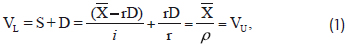
Where V_L= the market value of the levered firm, S = the market value of levered equity, D = the market value of riskless debt, = the expected value of risky stream that is divided between the firm's shareholders and debtholders as (-rD) and rD, respectively, r = the riskless debt rate, ρ = the expected market rate of capitalization with no taxes (i.e., required rate of return or cost of unlevered equity), i = the expected levered cost of equity with no taxes, and V_U = the market value of the unlevered (or no debτ) firm. Known as Proposition I, this no-tax model implies that the value of the firm is independent of its financial leverage and that unlevered and levered weighted average costs of capital (WACC) are equal to one another. Using equation (1), the value of equity can be computed alternatively as S = VL - D = VU - D. That is, given the value of unlevered equity, or V_U, we can substitute in values of debt, or D, within the range of 0 ≤ D ≤ VU to obtain the full range of equity values, or S.

With corporate taxes MM (1958, p. 272) originally posited that firm value is proportional to the expected after-tax earnings of the firm, or ^τ, as follows:

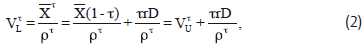
Where V_L = the market value of the levered firm after taxes, τ = the corporate tax rate, (1-τ) = the expected unlevered returns after taxes, ρ^τ= the appropriate after-tax market capitalization rate for unlevered equity, rD = the interest payments on riskless debt D paying the riskless debt rate r, and V_U^τ = the after-tax value of the unlevered firm. As already mentioned, modigliani (1988) later noted that, since the unlevered equity rate ρ^τ applied to discounting interest tax deductions trD is higher than the riskless debt rate r, the present value of the debt tax shield is substantially reduced.

In a major correction to their 1958 paper, MM (1963, p. 436) altered their original tax model by using the much lower riskless rate r to discount interest deductions. Discounting the expected after-tax earnings stream defined as now yielded the following firm valuation model: ⁸

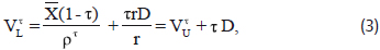
Where the tax gain is now D instead of rD/.⁹ MM created arbitrage proofs to show that, in equilibrium, levered firm value cannot be more or less than the sum of the unlevered firm value plus the tax gain D, such that equation (3) holds. The value of the firm is no longer proportional to its earnings after taxes, as firm value is dependent on the firm's capital structure. Indeed, excluding bankruptcy costs and other imperfections, their interpretation of this tax correction model was that the firm's shareholders will seek a corner solution of nearly all debt. The value of levered equity is computed simply as 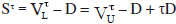, which shows that shareholders reap the large tax gain on debt interest. As in the original no tax valuation model, by varying the level of debt within the range 0 ≤ D ≤ V_L^τ, the full range of equity values, or S^τ, can be computed.

A comparison of alternative approaches to discounting interest deductions

In this section it is comparatively investigated how different discount rates used to find the present value of interest deductions affects equity and firm valuation results. To do this the cash flows paid out to shareholders is decomposed into their component parts. A portfolio approach is used to show that the equity rate is based on a weighted average of the component discount rates used to find the present values of the respective cash flow components paid to shareholders. According to MM's tax models, the riskiness of each cash flow component determines its appropriate discount rate. This logic explains the usage of the riskless rate in their tax correction model to discount interest deductions, which are considered riskless assuming the firm maintains a constant level of debt. As noted in the previous section, some authors assess the riskiness of interest deductions to be similar to free (unlevered) cash flows, which occurs upon relaxing the constant debt assumption to allow for a constant market value leverage ratio. In this case, consistent with MM's original tax model, interest deductions are discounted at the unlevered equity rate rτ.

In brief, portfolio analyses reveal that, when debt exceeds the unlevered value of the firm, component cash flows before interest deductions paid to shareholders imply negative equity values before interest deductions and associated negative equity discount rates. An alternative revised tax model is proposed that overcomes these problems by discounting each cash flow at the required rate of return of the particular investor actually receiving the cash flow. Thus, portfolio analyses imply that interest deductions paid out to shareholders should be discounted at the cost of equity i^τ.

Decomposing equity cash flows in MM's tax models

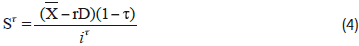
Since interest deductions are paid out to shareholders, focus is made on equity valuation effects of these potential tax gains. According to MM's tax correction model, the value of equity is:

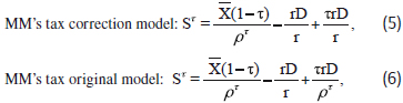
This general expression can be decomposed in different ways depending on the discount rates chosen for interest deductions. For example, MM's corrected and original tax models, respectively, decompose these cash flows using r and r^τ to discount interest deductions, respectively, as follows:

These decompositions can be proven from basic portfolio theory. Setting equations (4) and (5) equal to one another, the discount rate for the portfolio of shareholder cash flows (i.e., i^τ) is a weighted average of the discount rates (i.e., ρ^τ and r) associated with respective portfolio components. As shown in the appendix, the cost of equity can be solved to get

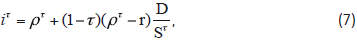
Which agrees with MM's formula in their tax correction model. Similarly, the cost of equity based on equations (4) and (6) yields

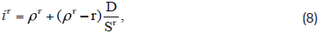
Which confirms MM's formula in their original tax model. These results validate the portfolio approach as a methodology for decomposing shareholder cash flows.

Another way to decompose shareholders' cash flows is to split them into the cash flow after taxes but before interest deductions equal to (1-τ) - rD plus interest deductions τrD. To find the discount rate to apply to the former cash flow, suppose that corporate taxes exist but there is no tax deductibility of interest and, therefore, no debt tax gain. Now shareholders' total cash flows equal (1-τ) - rD. In this realistic case¹⁰, it is obvious that MM's Proposition I in their original no-tax valuation model would hold. Defining V^τ_NTG= the levered value of the firm with taxes but no-taxgain (denoted NTG) and S^τ_NTG = the levered value of equity with taxes but no-tax-gain from interest deductions.

Proposition I implies that V^τ_NTG= S^τ_NTG + D = V^τ_U.¹¹ the present value of equity cash flows can be defined in this case as:

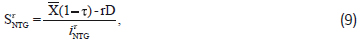
Where is the no-tax-gain cost of equity. Decomposing i^τ_NTG

These cash flows as follows:

We can solve for i^τ_NTG via the portfolio approach to get¹²

Using these results, shareholder cash flows in MM's tax models can be decomposed as

Because the equity component S^τ_NTG is common in both cases, these equations clearly show that equity value is affected by the choice of discount rate for interest deductions. Setting these equations equal to the more general equity expression in equation (4), the portfolio approach again yields the cost of equity equations (7) and (8) (see appendix for proof).

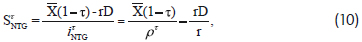
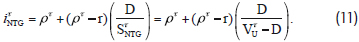
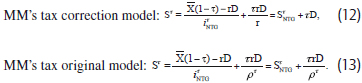
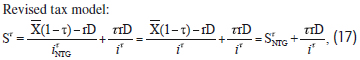
Based on these results, MM's tax correction model can be rewritten as:

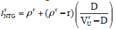
Where S^τ_NTG = V^τ_U at zero debt. This equation explicitly shows the well-known MM result that shareholders reap all tax gains on debt, i.e., S^τ = S^τ_NTG + τD. MM's original tax model yields . Notably, when debt levels reach the point at which D >V^τ_U, the levered equity value with no-tax-gain S^τ_NTG becomes negative in their valuation models. This negative equity value is confirmed by the negative cost of equity i^τ_NTG in equation (11) when D > V^τ_U. For example, given = 1, τ = 0.30, and ρ^τ = 0.10, such that V^τ_U = 1(1 - 0.30) / 0.10), and also given that D = 8 (i.e., D >V^τ_U), MM's tax correction model yields τD = 2.4, V^τ_L= V^τ_U + τD = 9.4, and S^τ = V^τ_L- D = 1.4, such that S^τ_NTG = S^τ-τD = V_U - D = -1 and i_NTG = 0.10 + (1-0.30)(0.10-0.04)8/-1 = -0.236. In this respect, whenever D > V_U, which occurs over a considerable debt range from V_U to the all debt value of firm at V^τ_Lmax= D_max = V^τ_U + τD_max, the value of S^τ_NTG will be negative. Of course, it is not possible for equity value to be negative, as it has a lower bound of zero due to limited liability of equity holders. Also, the expected cost of equity has a lower bound equal to the riskless rate and, therefore, cannot be negative.

To avoid these problems, if interest deductions are discounted at the cost of equity under the proposed revised tax model, S^τ_NTG and i^τ are not negative at any debt level. If this possibility is considered, shareholder cash flows can be decomposed as follows:

Using the portfolio approach to solve for the cost of equity (see appendix), we obtain¹³

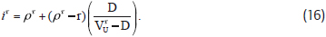
Interestingly, the cost of equity with interest deductions i^τ in equation (16) is the same as the cost of equity without interest deductions i^τ_NTG in equation (11). Consequently, it can be written that:

Where i^τ = i^τ_NTG. The revised tax model posits the following valuation relationships:

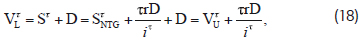
Which differs from MM's tax correction model in equation (14). Since the cost of equity increases at an increasing rate as the firm increases financial leverage, interest tax deductions will be considerably less than MM's tax model, especially at higher debt levels. The next section shows this effect by means of numerical examples. Importantly, it is found that S^τ_NTG and i^τ are not negative at any debt level.

A natural question is: When debt exceeds unlevered value in MM's tax models, which are derived under the assumption of interest deductibility, are there any real economic consequences of negative equity without interest deductions? to answer this question, suppose that interest is deductible from taxes but the government changes the tax rules to disallow such deductions. For firms with D > V^τ_U, the value of S^τ_NTG is negative, which would cause equity value to immediately fall to zero. In effect, all of equity value is simply due to debt tax gains. None of the operating profits of the firm contribute to equity value, which does not make sense under the assumption of no bankruptcy risk. For instance, suppose that = 1, τ = 0.30, ρ^τ = 0.10 (i.e., V^τ_U = (1 - τ)/ρ^τ = 1(1 - 0.30)/0.10 = 7), and r = 0.04. Under these assumptions, even at almost the maximum debt in MM's tax correction model, after-tax cash flows without interest deductions are sufficient to cover interest payments, or (1 - τ) > rD as 1(1 - 0.30) = 0.70 > 0.04(9.99) = 0.3996, where D = 9.99 at near the corner solution of all debt. Since there is no bankruptcy risk even at high debt levels, and operating profits are always positive, equity value with no interest deductions (and related cost of equity) should not be negative in their tax correction model without interest deductions.

In this section numerical examples are used to demonstrate the differences between MM's tax correction model and the proposed revised tax model. Table 1 compares the valuation results of these two models assuming that: v = 1, τ = 0.30, ρ = 0.04, ρ^τ = 0.10, and V^τ_U = 7 (i.e., V^τ_U = (1-τ)/ρ^τ = 1(1-0.30)/0.10 = 7). Referring to MM's tax correction model, it can be confirmed that S^τ = S^τ_NTG + τD; for example, at a debt/value ratio of 0.40, we have 4.77 ≅ 3.82 + 0.30(3.18). In this regard, the last column under MM's tax correction model results shows that, when D > V_^τU, the value of equity with no interest deductions, or S^τ_NTG becomes negative. By contrast, under the revised tax model, the value of debt does not exceed the unlevered value of the firm at any debt level, such that S^τ_NTG is never negative. Thus, discounting interest deductions at the cost of equity resolves the problem of negative equity without interest deductions found in MM's tax models.

Figure 1 plots data provided in table 1 to show that the levered cost of equity for the revised tax model¹⁴ (bold line) is somewhat higher than for MM's tax correction model (lower thin line). This result can be explained by the general expression for the levered cost of equity, or 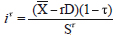wherein the value of equity in the denominator in the revised tax model is lower than in MM's tax correction model due to the lower debt tax gain available to shareholders.

A much larger disparity between these two models is apparent in Figure 2's valuation results. Note that, in contrast to MM's tax correction model, the value of debt in the revised tax model never exceeds the unlevered value of the firm, even at relatively high debt levels. As the capital structure approaches all debt, the tax gain trD/i^τ approaches zero, and debt approaches V^τ_U. Also, the revised tax model does not yield the all-debt corner solution of MM's tax correction model; instead, a flat-based, inverse U-shaped firm value function (bold line) emerges with a maximum firm value of 7.27 at an interior optimal debt/value ratio of about 0.55. This maximum firm value exceeds the unlevered value of the firm equal to 7 by only 0.27, which represents a debt tax shield of just 3.9 percent of unlevered equity value, as shown in the last column in table 1 labeled trD/i^τ. By comparison, at a debt/value ratio of 0.55, MM's tax correction model yields the much larger debt tax shield trD/r = tD of 1.38, or 19.7 percent of unlevered equity value. Additionally, the debt tax shield in MM's tax model continues to increase and even accelerate beyond this debt/value ratio. By comparison, the inverse U-shape of the firm value function in Figure 2 is relatively flat throughout the range of debt/value ratios. The flatness of the firm value function appears to support MM's (1958) Proposition I to some degree. Figure 3 shows the value of equity with no-tax-gain, or S^τ_NTG , in MM's tax correction model (bold line), which becomes negative when debt value exceeds the unlevered value of the firm, compared to its more compatible value in the revised tax model, which is always positive for any capital structure.

If a higher debt rate is assumed, the size of the debt tax shield increases to some extent. For example, all else the same, if the debt rate is raised to 0.08 (i.e., closer to the unlevered equity rate of 0.10), the maximum value of the firm increases to 7.80 at an optimal debt/value ratio of about 0.60. This optimal capital structure is not much different than the 0.55 optimal ratio at the 0.04 debt rate, which suggests that the optimum is relatively stable and would not change much in a dynamic setting. However, the debt tax shield jumps from 0.26 to 0.80, or from 3.9 percent to 11.4 percent of unlevered equity value, as the debt rate increases from 0.04 to 0.08. Hence, all else the same, changes in debt rates can cause the magnitude of the debt tax shield to noticeably change. Figure 4 graphs the valuation results using the higher riskless debt rate of 0.08, which shows that the debt tax shield is considerably higher than in Figure 1 (i.e., the firm value function in more inverse U-shaped). Sensitivity of debt tax shields to interest rates contrasts sharply with MM's tax correction model in which the present value of debt tax shields does not change as riskless debt rates increase. This result seems counter-intuitive, as higher riskless debt rates provide increasingly greater interest tax deductions that are available to shareholders, and vice versa.

What if the unlevered (rather than levered) cost of equity is used to discount all expected after-tax earnings of the firm including interest tax deductions as in MM's original tax model?¹⁵ Figure 5 repeats the above analyses under this assumption.¹⁶ The thin line represents MM's tax correction model. The bold lines graph MM's original tax model discounting debt tax shields at the unlevered cost of equity using riskless debt rates of 0.04 and 0.08, all else the same. At the lower riskless debt rate of 0.04, the maximum debt tax shield is about 0.95 at near all debt, but it in-creases considerably to about 2.21 at the higher debt rate of 0.08. Figure 5 shows that using the higher debt rate of 0.08 yields large tax gains on interest deductions that approach MM's tax correction model. Hence, as the spread between the unlevered cost of equity and riskless debt rate decreases (e.g., due to lower business risk for a firm or good economic times with lower general business risk that tend to lower the unlevered cost of equity), the difference in firm values between MM's original tax and tax corrected tax models decreases. These results demonstrate that discounting debt tax shields at the unlevered cost of equity: (1) still implies an all-debt capital structure, and (2) does not necessarily diminish debt tax gains to small values relative to MM's tax correction model under low business risk conditions. Moreover, using unlevered equity rates yields the same negative equity values as MM's tax correction model. Assuming that V^τ_U = 7 and d = 8 as in section 2 (i.e., D > V^τ_U), regardless of the riskless debt rates and unlevered equity rates used, we again obtain S^τ_NTG = V_^τU -D = -1. The only difference from MM's tax correction model is that the maximum value of debt is reduced due to the lower maximum firm value using the unlevered equity rate. Nonetheless, at some point debt value can exceed unlevered equity value, which implies negative equity value with no-tax-gains.

Not surprisingly, the cost of capital under the revised tax model differs considerably from MM's tax correction model but is similar to their original tax model. The weighted average cost of capital for a levered firm can be generally¹⁷ defined as:

Where r(1- τ) = the after-tax cost of debt. Substituting the levered cost of equity in equation (16) into equation (19), the WACC can be written as:

If the levered equity rate i^τ is replaced with the riskless debt rate r, MM's tax correction model's cost of capital, or WACC = (1-τ D_L/V^τ_L), is obtained. Equation (20) implies that, as the riskless debt rate increases, the cost of capital function becomes more U-shaped (and related firm value function more inverse U- shaped), all else the same. Figure 6 plots the cost of capital for the revised tax model in equation (20) versus MM's tax correction model using data from Table 1's numerical examples. The cost of capital for MM's tax correction model falls continuously until it reaches a relatively low minimum at all debt, where firm value is maximized. However, the minimum cost of capital for the revised tax model is slightly U-shaped with a minimum value of about 0.096 at an optimal debt/value ratio of about 0.55, where firm value is maximized at 7.27. The relatively flat shape of the cost of capital function is again somewhat consistent with MM's Proposition I. The fact that the cost of capital does not decrease substantially as more low cost debt is employed by the firm is attributable to discounting interest tax deductions at the levered cost of equity, which is evident in equation (20). Increased debt results in higher interest tax deductions but a higher levered cost of equity also.

Miller's (1977) renowned work on capital structure, firm valuation, and personal taxes proposed dramatically lower debt tax shields compared to MM's tax correction model.¹⁸ This section extends the revised tax model to the Miller valuation model incorporating both corporate and personal taxes. Tax terms are defined as follows: τps = the personal tax rate on equity earnings, τpb = the personal tax rate on debt earnings, and q = [1- (1-τ)(1-τps)/(1-τpb)]. According to Miller, due to equilibrium tax conditions in the bond markets, the value of the firm with corporate and personal taxes is V^τ_L=V^τ_U + θD. Particularly relevant to the present paper, cash flows to shareholders are exposed to personal equity tax rates as follows:

,

Where the last term clearly shows that the interest tax deductions are shareholders' cash flow due to its association with the personal equity tax rate (per Ross' observation cited earlier).

Given that ρ^π is the unlevered cost of equity after both corporate and personal equity taxes, the levered cost of equity in the revised tax model becomes

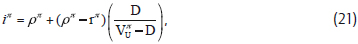
Where the debt rate is after personal taxes on debt interest, and after-tax values are denoted by superscript π. The value of the firm becomes

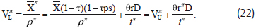
With no personal taxes, equations (21) and (22) collapse to their corporate tax only counterparts in equations (16) and (18), respectively.

Under Miller's equilibrium corporate and personal tax conditions wherein θ = 0, the debt tax shield is zero and equation (22) collapses to the no-tax-gain relation V^τ_NTG = S^τ_NTG + D = V^τ_U, such that Proposition I holds as proposed earlier in section 2. However, if θ ≠ 0 for an individual firm, then leverage changes the value of the firm. Since it is likely for individual firms that θ < τ, previous results for the revised tax model under low tax rates are most applicable. Thus, conditional on the assumption that the spread between the unlevered cost of equity and debt rate is not relatively low, Proposition I generally holds for low levels of q for an individual firm but may be rejected as q increases. Also, even if θ = τ due to national tax policies (e.g., for τ = τps = τpb or other tax regimes), Proposition I can approximately hold under conditions discussed in the previous section. Hence, while Miller's introduction of personal taxes substantially affects MM's tax model valuation results, personal taxes do not change the form of the revised tax model and have much less effect on the valuation results. For the most part, the revised tax model is robust to the introduction of personal taxes, which lends further support for its predictions.

The revised tax model has a number of important implications to corporate capital structure decisions and related literature that tend to affirm its feasibility as a plausible valuation theory. First, the revised model implies much smaller debt tax shields than MM's original and tax correction models. In the comparative examples in table 1, given an unlevered equity value of 7, the maximum debt tax shield is 0.27 compared to the maximum of 3 for MM's tax correction model at all debt. In the context of the tradeoff theory balancing expected tax gains on interest deductions against expected bankruptcy costs, the revised tax model implies a "fox and rabbit stew," in contrast to Miller's (1977) observation that MM's tax correction model envisages a "horse and rabbit stew." Consistent with modest debt tax gains, a number of U.s. And international empirical studies (e.g., MacKie-Mason (1990), Rajan and Zingales (1995), Booth, Aivazian, Demirgüç-Kunt (2001), Huizinga, Laeven, Nicodeme (2008), and others) have confirmed that the relationship between firm leverage and taxation is relatively weak. Also, a number of studies have found that debt tax benefits have a smaller effect on firm value than MM's tax correction would predict (e.g., Fama and French (1998), Graham (2000, 2008), Kemsley and Nissim (2002), and others). For example, Graham (2000) found that the tax benefit of debt is about 9-10 percent of firm value in the period 1980-1994. Kemsley and Nissim (2002) estimated the value of the net debt tax shield for U.S. firms in the period 1963-1993 to be about 10 percent of firm value. Another study by Graham (2008) provided a range of debt tax benefits relative to firm value from 7.7 percent to 9.8 percent in the period 1995-1999. Recently, van Binsbergen, Graham, and Yang (2010) appraised the net benefit of debt to be about 3.5 percent of firm value (i.e., a 10.4 percent gross benefit and 6.9 percent costs), and Korteweg (2010) assessed the net benefits of debt to be about 5.5 percent of firm value. Using data from table 1 (see Figure 1) with the debt rate set at 0.04, MM's maximum debt tax shield at near all debt approaches 30 percent of firm value, whereas we get a maximum of only 3.7 percent at a debt/value ratio of 0.55. However, upon increasing the debt rate from 0.04 to 0.08 (see Figure 2), the maximum tax shield for the revised tax model is slightly more than 10 percent of firm value at a debt ratio of 0.60. Using this higher debt rate, Figure 7 compares the present values of debt tax shields (in percent of firm value terms) for MM's tax correction model and our revised tax model. Our results for debt rates in the range of 0.04 to 0.08 are remarkably consistent with empirical evidence.

In this regard, no bankruptcy are assumed costs in deriving our debt tax shield. However, bankruptcy and other balancing costs are impounded in debt and equity rates, as debtholders and equityholders adjust their expected rates of return to reflect such costs. Consequently, balancing costs should not change the form of the revised tax model's valuation results. Equation (16) shows that the cost of equity would be affected by balancing costs via their impact on the debt rate. Bankruptcy risk would increase the debt rate, as bondholders demand a risk premium to compensate for potential future losses of interest and principal. As the debt rate increases and becomes closer to the unlevered equity rate, potential debt tax shields tend to increase (as discussed previously with respect to Figure 4). Other variables in the equation, including the unlevered equity rate, debt, and equity, would be based on market values. Using the cost of equity to discount firms' interest tax deductions provides a simple way to capture how investors exposed to bankruptcy and other risks value debt tax shields. Empirical tests can readily implement this approach to quantify net tax shields on debt interest deductions and observe the tax shield function throughout the range of observed leverage.

Second, the results in table 1 indicate that there is a fairly wide range of debt/value ratios within which most of the present value of debt tax shields is captured. For example, when 0.30 < (D_L/V^τ_L< 0.80, the debt tax gains available to shareholders reach levels in the range of 0.18 to 0.27 assuming r = 0.04 and in the range of 0.49 to 0.80 assuming r = 0.08. It appears that differences in the levels of debt tax shields within this debt/value range are relatively small, especially for lower riskless debt rates relative to unlevered equity rates. It is inferred that the revised tax model implies a "relevant range" for capital structure in the sense that most tax gains available to shareholders are achieved. This implication agrees with empirical evidence and actual practice. In this regard, Kane, Marcus, and Mcdonald (1984) have reported that the actual range of debtto-value ratios for U.S. firms is from zero to 60 percent. More recently, Frank and Goyal (2008) have documented that the average debt-to-value ratios of the aggregate U.s. nonfarm, nonfinancial business sector ranged from 0.27 to 0.45 in the period 1945 to early 2000s. Related to this discussion, the revised tax model implies that even moderate debt-to-value ratios are able to capture the lion's share of shareholder tax gains. Hence, it is possible that debt-to-value ratios could vary considerably among similar firms that obtain most tax gains available to shareholders - an implication that helps to mitigate a previously unaddressed problem in the static trade-off theory of capital structure observed by myers (1984).

Third, the revised tax model implies that even firms with low probabilities of financial distress and, in turn, low expected bankruptcy costs may employ fairly conservative debt-to-value ratios. This implication helps to reconcile another problem inherent in the trade-off theory raised by myers (2001). That is, many highly profitable and big firms with investment grade credit ratings use conservative levels of debt even though the trade-off theory predicts that such firms should use higher levels of interest tax shields (e.g., Graham (2000, 2008), Kemsley and Nissim (2002), and others).¹⁹ in view of the revised tax model, even firms with no expected bankruptcy costs would not likely use high levels of interest tax shields. Most tax gain advantages of debt are exhausted in the lower half of the relevant debt/value range.

Fourth, the revised tax model implies an inverse U-shaped firm value function. The hallmark of the trade-off theory balancing debt tax gains against expected bankruptcy and other potential debt-related costs is an inverse U-shaped firm valuation function. However, the revised tax model yields this intuitively attractive and popular firm valuation function without these balancing costs. It is the nonlinearly increasing levered cost of equity as debt increases that serves as a countervailing force to offset rising interest deductions and produce the inverse U-shaped firm value function. Additionally, introducing bankruptcy costs in a trade-off valuation setting can be readily implemented by appropriately adjusting the levered cost of equity.

Fifth, returning to the impact of changes in riskless debt rates discussed in the previous section, as riskless debt rates increase relative to a fixed unlevered cost of equity, Figure 4 shows that debt tax shields increase and optimal debt/value ratios are somewhat higher than for lower riskless debt rates in Figure 2, all else the same. In the limit at a zero interest rate, there is no debt tax shield, and the value of the firm is independent of financial leverage in line with Proposition I of MM's original no tax model. It can be inferred that, as riskless debt rates fall to very low levels that approach zero, trivial debt tax shields imply that Proposition I holds for the most part. On the other hand, as riskless debt rates increase narrowing the difference from the unlevered cost of equity, the debt tax shield function becomes more inverse U-shaped indicative of significant potential debt tax shields and, therefore, rejection of Proposition I. Hence, the revised tax model may or may not reject Proposition I depending on the level of riskless debt rates (relative to the unlevered cost of equity) that affects the shape of the firm value function. Starkly contrasting with these riskless debt rate implications, in MM's tax correction model very low interest rates have no effect on debt tax shields (i.e., equal to td for all positive riskless debt rates even if the magnitude of interest deductions is trivial). The same problem affects discounting debt tax shields with the unlevered equity rate in the case of firms with low business risk that have unlevered equity rates close to the riskless rate.

Sixth, assuming a fixed riskless debt rate, the revised tax model results in Figures 2 and 4 imply that firms with higher business risk have lower debt tax shields and optimal debt/value ratios, all else the same. Higher business risk increases the unlevered cost of equity and, therefore, widens its spread over the fixed riskless debt rate. Conversely, firms with lower business risk have narrower spreads between the unlevered cost of equity and riskless debt rate, which makes the firm value function more inverse U-shaped. Following this logic, in good economic times with lower general business risk, the present value of the debt tax shield would be more inverse U-shaped across firms, and vice versa in bad economic times (i.e., unlevered equity rates increase in recessions and riskless debt rates tend to decrease due to stimulative monetary policy efforts by central banks, which would increase their spread and tend to flatten the firm value function). It can be inferred that Proposition I is more likely to hold for high than low business risk firms and for bad as opposed to good economic times. Also, differences between high and low business risk firms decrease as riskless debt rates de-crease and are virtually eliminated as riskless debt rates and therefore debt tax shields approach zero as observed above. It is possible that differences in business risk help to explain the fact that leverage ratios of low and high debt firms are highly persistent over time and not related for the most part to size, profitability, market-to-book, industry, and other previously identified determinants of capital structure (see Titman and Wessels (1988), Rajan and Zingales (1995), Mackay and Phillips (2005), Lemmon, Roberts, and Zender (2008), and citations therein).

Seventh, the debt tax shield function is affected by the corporate tax rate. As corporate tax rates increase, the debt tax shield available to shareholders increases, all else the same (i.e., (τrD/i^τ)/τ > 0). This tax effect on corporate capital structure is consistent with empirical work by MacKie-Mason (1990), Trezevant (1992), Graham (1996), and Graham, Lemmon, and schallheim (1998), who have found that high-tax-rate firms use more debt than low-tax-rate firms. Also, other papers by Gordon and MacKie-Mason (1990), Givoly, Hahn, ofer, and Sarig (1992), Rajan and Zingales (1995), Booth, Aivazian, Demirgüç, Maksimovic (2001), and Huizinga, Laeven, and Nicodeme (2008) have found that changes in corporate (and personal) tax rates lead to predicted changes in debt ratios among firms.

Eighth, the revised tax model with personal taxes implies that Proposition I is more likely to hold, which may help to explain the weak effect of national tax regimes on firm leverage found in international empirical studies by Rajan and Zingales (1995), Booth, Aivazian, Demirgúç, Maksimovic (2001), Huizinga, Laeven, and Nicodeme (2008), and others.

Ninth, and last, a general implication based on the above discussion is that Proposition I can approximately hold under a variety of conditions, including relatively low riskless debt rates, high unlevered costs of equity (i.e., business risk), and low corporate tax rates, as well as combinations of these conditions. An inverse U-shaped firm value function exists but its shape is relatively flat under these conditions. This general implication is consistent with Modigliani's (1988) later reversal of the 1963 MM tax correction model in favor of Proposition I in the original 1958 MM paper. Under other conditions, Proposition I may not hold. Perhaps the most obvious assumption to relax is riskless debt. Most firms issue debt at an interest rate in excess of comparable maturity government debt (e.g., U.S. treasury rates). These higher debt costs would tend to boost interest tax deductions as well as narrow the spread from unlevered equity rates and, therefore, work against Proposition I.

Together, the aforementioned implications lend support for the revised tax model by helping to reconcile theory and evidence on capital structure and firm valuation. Of course, future empirical tests are recommended to directly investigate the tax shield function hypothesized by our revised tax model.

MM corrected their 1958 debt irrelevance proposition in 1963 to derive an all debt corner solution to capital structure. In efforts to soften this extreme outcome, researchers have introduced bankruptcy and other potential debt costs as balancing factors, relaxed the no personal taxes assumption, and discounted interest tax deductions using different debt and unlevered equity rates.

Given that their tax models imply that after-tax equity value equals the sum of the after-tax equity value with no interest deductions (denoted S^τ_NTG) plus the tax gain on interest deductions, it is found that equity value S^τ_NTG becomes negative (as well as the associated cost of equity i^τ_NTG) when debt levels exceed the unlevered value of the firm. Of course, negative equity values and equity rates are not possible.

An alternative discounting approach for debt tax shields was proposed that resolves these issues. Portfolio analyses showed that that the cost of equity with and without interest deductions is the same and does not become negative at any debt level. Also, it was found that the equity value component S^τ_NTG is never negative. These findings suggest that, because interest deductions are paid out to shareholders, they should be discounted at the cost of equity. Shareholders discount all of their cash flow components, whether from riskless or risky sources, at the appropriate cost of equity. In this regard, shareholders value their cash flows by decomposing them into unlevered equity cash flows discounted at the unlevered equity rate plus levered cash flows (viz., interest deductions) discounted at the levered equity rate.

The main findings of the proposed revised tax model are plausibly consistent with empirical evidence: (1) much smaller debt tax shields than in MM's original and tax correction models; (2) a flat-based, inverse U-shaped firm value function with an interior optimal capital structure as opposed to an all-debt corner solution; (3) a relevant range of debt/value ratios spanning a fairly broad interval within which most debt tax shields are captured; (4) a flatbased U-shaped cost of capital function; and (5) debt tax shields and optimal capital structures that are sensitive to riskless debt rates, unlevered costs of equity (i.e., business risk), and corporate tax rates. These results appear to be more akin to real world capital structure. Interestingly, under some discount rate conditions, the firm value function is almost flat as leverage increases, which supports to some extent MM's original 1958 Proposition I that firm valuation is independent of capital structure. However, as these variables interact to produce higher debt tax shields that are economically meaningful to shareholders, Proposition I was rejected.

The revised tax model helps to explain the relatively weak relationship between financial leverage and national tax policies reported by numerous empirical studies. Also, it addresses some previous criticisms of the trade-off theory of capital structure by Miller (1977), myers (1984, 2001), and others rooted in large tax gains under MM's tax correction model relative to expected bankruptcy costs. With respect to these criticisms, comparative static analyses of shareholder tax gains suggested that: (1) Miller's criticism of MM's tax correction model as a "horse and rabbit stew" can be less severely described as a "fox and rabbit stew;" (2) it is possible that similar firms could have widely divergent leverage ratios; and, (3) large and profitable firms with low probabilities of financial distress may reasonably utilize fairly conservative debt-to-value ratios. Graham (2003, 2008) has cited the latter "underlevered or conservative leverage puzzle" as an unresolved issue in capital structure. In this regard, the debt tax shield results of this paper do not support aggressive use of leverage even for large, profitable firms with low business risk (even though they have greater potential debt tax shields than high business risk firms) and, therefore, help to explain more moderate approaches to corporate debt financing observed in the real world. Based on these findings and implications, relevant to Green and Hollifield's (2003) criticism of the MM tax correction model noted earlier in section 1, it is concluded that MM's tax model in our proposed revised form should play a greater role in corporate capital structure pedagogy and policy than previously believed.

Reflecting on his approach to introducing imperfect information in economic models of competition, stiglitz (2001, p. 519) observed that, "it is not easy to change views of the world, and it seemed to me the most effective way of attacking the paradigm was to keep within the standard framework as much as possible." likewise, the present paper has sought to stay within MM's comparative-static valuation paradigm, rather than using option-based, dynamic, or other valuation approaches.

Since the revised tax model predicts that the present value of debt tax shields is not large, other factors potentially affecting firm value, including bankruptcy costs, agency costs, asymmetric information, non-debt tax shields, market timing, corporate control, debt heterogeneity, bank credit, etc., are relatively important to capital structure decisions by firms (e.g., for citations and discussion of this extensive literature, see Graham (2003, 2008), and Hovakimian, Hovakimian, and tehranian (2004)). How these other factors precisely affect the inverse U-shaped debt tax shield function and the dynamic effects of changing corporate and personal tax rates, debt rates, and unlevered equity rates (business risk), in addition to changing debt levels, expected bankruptcy costs, and other factors, on the debt tax shield function are left for future study. While revised tax model analyses clearly suggest that optimal capital structures will be little affected by such dynamics, the magnitude of the debt tax shield may well be affected. Finally, from a policy perspective, if excessive financial leverage in the 1990s and 2000s, especially in the home and commercial mortgage markets, was motivated in part by the desire of market participants to capture large debt tax gains, the revised tax model suggests that such efforts were misguided.

Acknowledgments

Benefit has been received from numerous discussions over the years with many colleagues, including Ali, Anari, Will Armstrong, Jaap Bos, Michele Caputo, Paige Fields, Donald Fraser, Johan Knif, Michael Koetter, Seppo Pynnönen, Joseph Reising, Hwan Shin, Soenke Sievers, Sorin Sorescu, Antti Suvanto, Joseph Tham, and Marilyn Wiley, in addition to participants at the 2008 Financial management association european conference in Prague, Czech Republic, 2010 midwest Finance Conference in Las Vegas, Nevada, and 2010 international Finance Conference in Mexico City, Mexico. All remaining errors are the responsibility of the authors.

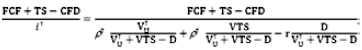
This appendix applies a portfolio approach to equity discount rates and their component cash flows. Three alternative cases are considered using the riskless debt rate r, unlevered equity rate ρ^τ, and cost of equity i^τ to discount interest deductions available to shareholders. Shareholders cash flows are defined as CFE = ( - rD)(1 - τ) which is comprised of free cash flow FCF = (1-τ) interest tax shields TS = τrD, and cash flow to debtholders CFD = rD, i.e., CFE = FCF + TS - CFD. Lastly, we also consider the case in which no interest deductions are allowed, such that shareholders' cash flow is CFBI = FCF - CFD plus interest deductions TS.

First, assuming ts is discounted using the riskless debt rate r as in MM's tax correction model, the cost of equity i^τ can be solved as follows. From a portfolio perspective, the cost of equity is a weighted average of the discount rates associated with component cash flows, or

Where VTS = the present value of interest deductions discounted at r, and V_^τU + VTS - D = the value of equity. Rearranging this equation,

Since VTS = τD in the case of discounting interest deductions at the riskless rate r, we get i^τ = ρ^τ + (1 - τ)(ρ^τ - r)D/ S^τ, which is the same as MM's tax correction formula.

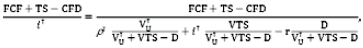
Second, assuming ts is discounted using the unlevered equity rate as in MM's original tax model, the portfolio approach implies the following decomposition:

Following the same steps as before, we obtain i^τ = ρ^τ + (ρ^τ- r) D/ S^τ, which agrees with MM's formula.

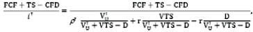
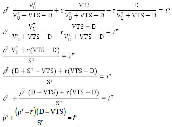
Third, assuming that ts is discounted using the cost of equity under the proposed revised tax model, the following decomposition of cash flows is obtained:

Which can be solved to obtain i^τ = ρ^τ +(ρ^τ - r)D/( V^τ_U - D) as in equation (16) in the text.

Fourth, and last, shareholders' cash flow components can be redefined as comprised of cash flows before interest deductions, denoted CFBI = FCF - CFD, plus interest deductions TS. Using r to discount interest deductions under MM's tax correction model, the portfolio approach suggests that:

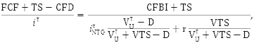
Where V^τ_U - D in the denominator of the right-hand-side equals S^τ_NTG, or the no-tax-gain value of equity. After substituting

From equation (11) in the denominator and rearranging terms, we again obtain MM's result i^τ = ρ^τ +(1 - τ)(ρ^τ - r)D/S^τ. This same procedure can be repeated by discounting interest deductions using the unlevered equity rate or the cost of equity to yield MM's original tax model or revised tax model formulas defined above, respectively.

¹ We have benefited from numerous discussions over the years with many colleagues, including Ali, Anari, Will Armstrong, Jaap Bos, Michele Caputo, Paige Fields, Donald Fraser, Johan Knif, Michael Koetter, Seppo Pynnönen, Joseph Reising, Hwan Shin, Soenke Sievers, Sorin Sorescu, Antti Suvanto, Joseph Tham, and Marilyn Wiley, in addition to participants at the 2008 Financial Management Association European conference in Prague, Czech Republic, 2010 Midwest Finance Conference in Las Vegas, Nevada, and 2010 International Finance Conference in Mexico City, Mexico. All remaining errors are the responsibility of the authors.

² For example, see Myers (1974), DeAngelo and Masulis (1980), Masulis (1980), Fama and French (1998), Ruback, (1995, 2002), Graham (2000, 2008), Graham and Harvey (2001), Brealey and Myers (2003), Arzac and Glosten (2005), and many others. Graham (2003) provides an excellent review of this literature.

³ For studies debating different discount rates, see miles and ezell (1980, 1985), Harris and Pringle (1985), modigliani (1988), damodaran (1994), Kaplan and Ruback (1995), Ruback (2002), Fernandez (2004, 2007), arzac and Glosten (2005), Cooper and nyborg (2006), and others. For example, miles and ezell (1985) have argued that, if firms maintain a constant level of debt as assumed by MM, the riskless cost of debt is the appropriate discount rate for the debt tax shield. However, if firms instead maintain a constant debtto-firm value ratio, debt tax shields should be discounted using the unlevered equity rate.

⁴ standard textbooks in finance commonly note that interest tax deductions increase the cash flows of shareholders. For example, Grinblatt and titman (1998, p. 511) observe that, if a firm issues debt to buy back equity, remaining shareholders benefit from an increase in cash flow associated with interest tax deductions on debt.

⁵ simple numerical examples are available from the authors upon request.

⁶ See also Gordon (1989) and Weston (1989).

⁷ Stiglitz (1969) has shown that MM's original valuation model with no taxes holds under more general conditions, in such a way that these assumptions are not restrictive for the most part.

⁸ it is assumed in this model that debt is constant. A s shown later, a constant debt policy can be expressed as a constant leverage ratio policy also.

⁹ see myers (1974), miles and ezzell (1980, 1985), Fernandez (2004), and Cooper and nyborg (2006) for discussion and different viewpoints on computing the present value of tax shields.

¹⁰ According to Warren (1974), interest deductions for U.S. corporations in the 1800s and early 1900s were quite limited and generally disallowed. in 1918 unlimited interest deductions were temporarily allowed by Congress to offset the World War I excess profits tax. When this tax was repealed in 1921, interest deductions were retained with no explanation given by Congress. Relevant to the present discussion, historical precedent exists for the plausibility of not allowing firms to deduct interest from earnings. more recently, due to budget deficit concerns, some legislative proposals in the U.s. Congress call for the elimination of interest deductions on home mortgage loans. if such a tax loophole was closed for homeowners, it would seem conceivable that corporate interest deductions from federal income taxes could be reduced or eliminated also.

¹¹ As noted in Section 4, Miller's equilibrium corporate and personal tax conditions similarly imply that there is no debt tax gain, so that Proposition i holds.

¹² This cost of equity formula is the same as MM's no-tax cost of equity but on an after-tax basis.

¹³ an alternate cash flow proof of equation (16) is to assume that Ψ vts = ts, where Ψ = the discount rate on debt interest tax deductions, vts = the present value of the debt tax shield, and ts = the interest tax deduction in each period. We can similarly define the cash flows available to shareholders (CFe), debtholders (CFd), and the unlevered firm (FCF) as i^t S^t = CFe, r d = CFd, and V_U = FCF, respectively. Using these definitions, the cash flows of the firm can be written as FCF + ts = CFe + CFd or V_U + Ψ vts = i^t S^t + r d. if we assume ψt = i^t, then we have V_U+ i^t vts = i^t S^t + r d, which can be readily solved to get i^t in equation (16). Based on the adjusted Present value (aPv) approach, this result can easily be shown to hold for both perpetuities and finite cash flows. Unlike MM's cost of equity formulas, notice that levered equity value does not show up on the right-hand-side. since the cost of equity i^t depends on the value of equity s^t, and vice versa, in their formulas, there is circularity between i^t and s^t (see miles and ezzell (1980, p. 729)). By contrast, no such circularity exists in equation (16) for fixed d.

¹⁴ the levered cost of equity was computed using equation (11) and then checked against the general levered cost of equity formula, or i = (X -rD)(1)/S .

¹⁵ Kaplan and Ruback (1995) dubbed discounting all capital cash flows available to both debt and equity holders at the unlevered cost of equity the Compressed adjusted Present value technique (Compressed aPv). the intuition is that capital cash flows are comprised of all after-tax cash flows, including interest tax deductions. they noted that this approach is equivalent to the adjusted Present value (aPv) method of discounting interest tax deductions at the unlevered cost of equity. this approach assumes that interest tax deductions have the same systematic risk as the firm's unlevered cash flows, which are associated with the business risk of the firm.

¹⁶ the complete numerical example is available from the authors upon request.

¹⁷ this formula is popular in finance textbooks. its assumptions are not always met (e.g., operating earnings are greater than financial expenses, and taxes are paid the same year of accrual).

¹⁸ see also Benninga and sarig (1997) and Benninga (2006) for further discussion of personal taxes and debt tax shields.

¹⁹ Problems with the trade-off theory in part motivated myers (1984) to propose the pecking order theory of capital structure (see also myers and majluf (1984)). this theory predicts that firms do not have target or optimal capital structures. instead, driven by adverse selection costs derived from asymmetric information between managers and the financial market as well as debt capacity, firms initially utilize internally generated funds, then debt, and lastly equity in a pecking order. A nother theory of capital structure with no target leverage ratio focuses on market timing. Baker and Wurgler (2002) find that firms time equity issues to take advantage of high market values, which affect firms' short- and long-run capital structures.

Andrade, G. & Kaplan, S. N. (1998). How costly is financial (not economic) distress? Evidence from highly levered transactions that became distressed. Journal of Finance, 53(5), 1443-1493.         [ Links ]

Arzac, E. R. & Glosten, L. R. (2005). A reconsideration of tax shield valuation. European Financial Management, 11(4), 453-461.         [ Links ]

Baker, M. & Wurgler, J. (2002). Market timing and capital structure. Journal of Finance, 57(1), 1-32.         [ Links ]

Benninga, S. & Sarig, O. (1997). Corporate Finance: A Valuation Approach. New york: McGraw-Hill.         [ Links ]

Benninga, S. (2006). Principles of Finance with Excel. New york: Oxford University Press.         [ Links ]

Booth, L., Aivazian, V., Demirgüç, A. & Maksimovic, V. (2001). Capital structures in developing countries. Journal of Finance, 56(1), 87-130.         [ Links ]

Bradley, M., Jarrell, G. & Kim, E. H. (1984). On the existence of an optimal capital structure. Journal of Finance, 39(3), 857-878.         [ Links ]

Brealey, R. A. & Myers, S. C. (2003). Principles of Corporate Finance. New York: McGraw-Hill.         [ Links ]

Chen, A. H. & Kim, E. H. (1979). Theories of corporate debt policy: A synthesis. Journal of Finance, 34(2), 371-384.         [ Links ]

Cooper, I. A. & Nyborg, K. G. (2006). The value of tax shields IS equal to the present value of tax shields. Journal of Financial Economics, 81(1), 215-225.         [ Links ]

Damodaran, A. (2006, 2^nd ed.). Damodaran on Valuation. New york: John Wiley & Sons.         [ Links ]

Deangelo, H. & Masulis, R. (1980). Optimal capital structure under corporate and personal taxation. Journal of Financial Economics, 8, 3-29.         [ Links ]

Fama, E. & French, K. (1998). Taxes, financing costs, and firm value. Journal of Finance, 53(3), 819-843.         [ Links ]

Fernandez, P. (2004). The value of tax shields is not equal to the present value of tax shields. Journal of Financial Economics, 73, 145-165.         [ Links ]

Fernandez, P. (2007). A more realistic valuation: adjusted present value and WACC with constant book leverage ratio. Journal of Applied Finance, 17(2), 13-20.         [ Links ]

Frank, M. Z. & Goyal, V. K. (2008). Trade-off and pecking order theories of debt. In B. Espen eckbo (ed.), Handbook of Corporate Finance: Empirical Corporate Finance. North-Holland: Elsevier, Handbooks in Finance series, vol. 2.         [ Links ]

Givoly, D., Hahn, C., Ofer, A. & Sarig, O. (1992). Taxes and capital structure: Evidence from firms' response to the Tax Reform Act of 1986. Review of Financial Studies, 5, 331-355.         [ Links ]

Gordon, M. J. (1989). Corporate finance under the MM theorems. Financial Management, 18(2), 19-28.         [ Links ]

Gordon, R. H. & MacKie-Mason, J. K. (1990). Effects of the Tax Reform act of 1986 on corporate financial policy and organizational form. In J. Slemrod (ed.), Do Taxes Matter?, (pp. 91-131). Cambridge: MIT Press.         [ Links ]

Graham, J. R. (1996). Debt and the marginal tax rate. Journal of Financial Economics, 41(1), 41-73.         [ Links ]

Graham, J. R. (2000). How big are the tax benefits of debt? Journal of Finance, IV(5), 1901-1941.         [ Links ]

Graham, J. R. & Harvey, C. R. (2001). The theory and practice of corporate finance: Evidence from the field. Journal of Financial Economics, 60, 187-243.         [ Links ]

Graham, J. R. (2003). Taxes and corporate finance: A review. Review of Financial Studies, 16, 1075-1128.         [ Links ]

Graham, J. R. (2008). Taxes and corporate finance. In B. Espen Eckbo (ed.), Handbook of Corporate Finance: Empirical Corporate Finance. North-Holland: Elsevier, Handbooks in Finance series, vol. 2.         [ Links ]

Graham, J. R., Lemmon, M. & Schallheim, J. (1998). Debt, leases, taxes, and the endogeneity of corporate tax status. Journal of Finance, 53, 131-162.         [ Links ]

Green, R. C. & Hollifield, B. (2003). The personal-tax advantages of equity. Journal of Financial Economics, 67, 175-216.         [ Links ]

Grinblatt, M. & Liu, J. (2008). Debt policy, corporate taxes, and discount rates. Journal of Economic Theory, 141(1), 225-254.         [ Links ]

Grinblatt, M. & Titman, S. (1998). Financial markets and Corporate strategy. New york: McGraw-Hill.         [ Links ]

Harris, R. S. & Pringle, J. (1985). Risk-adjusted discount rates: extensions from the average risk case. Journal of Financial Research, 8, 237-244.         [ Links ]

Hovakimian, A., Hovakimian, G. & Tehranian, H. (2004). Determinants of target capital structures: the case for dual debt and equity issues. Journal of Financial Economics, 71, 517-540.         [ Links ]

Huizinga, H., Laeven, L. & Nicodeme, G. (2008). Capital structure and international debt shifting. Journal of Financial Economics, 88(1), 80-118.         [ Links ]

Kane, A., Marcus, A. J. & McDonald, R. L. (1984). How big is the tax advantage of debt? Journal of Finance, 39(3), 841-853.         [ Links ]

Kaplan, S. & Ruback, R. S. (1995). The valuation of cash flow forecasts: An empirical analysis. Journal of Finance, 50(4), 1059-1093.         [ Links ]

Korteweg, A. (2010). The net benefits of leverage. Journal of Finance, 65(6), 2137-2170.         [ Links ]

Kraus, A. & Litzenberger, R. H. (1973). A state-preference model of optimal financial leverage. Journal of Finance, 28(4), 911-922.         [ Links ]

Kemsley, D. & Nissim, D. (2002). Valuation and the debt tax shield. Journal of Finance, 57(5), 2045-2073.         [ Links ]

Lemmon, M. L., Roberts, M. R. & Zender, J. F. (2008). Back to the beginning: Persistence and the cross-section of corporate capital structure. Journal of Finance, 63(4), 1575-1608.         [ Links ]

Luehrman, R. (1997). Using APV: A better tool for valuing operations. Harvard Business Review, 75, 145-154.         [ Links ]

Mackay, P. & Phillips, G. (2005). How does industry affect firm financial structure? Review of Financial Studies, 18(4), 1433-1466.         [ Links ]

MacKie-Mason, J. K. (1990). Do taxes affect corporate finance decisions? Journal of Finance, 45(5), 1471-1493.         [ Links ]

Masulis, R. W. (1980). Stock repurchase by tender offer: An analysis of the causes of common stock price changes. Journal of Finance, 35(2), 305-319.         [ Links ]

Miles, J. & Ezzell, J. R. (1980). The weighted average cost of capital, perfect capital markets, and project life: a clarification. Journal of Financial and Quantitative Analysis, 15(3), 719-730.         [ Links ]

Miles, J. & Ezzell, J. R. (1985). Reformulating the tax shield: A note. Journal of Finance, 40(5), 1485-1492.         [ Links ]

Miller, M. (1977). Debt and taxes. Journal of Finance, 32(2), 261-275.         [ Links ]

Miller, M. (1988). The modigliani-Miller propositions after thirty years. Journal of Economic Perspectives, 2(4), 99-120.         [ Links ]

Modigliani, F. & Miller, M. H. (1958). The cost of capital, corporation finance and the theory of investment. American Economic Review, 48(3), 261-297.         [ Links ]

Modigliani, F. & Miller, M. H. (1963). Corporate income taxes and the Cost of Capital: a Correction. The American Economic Review, 53(3), 433-443.         [ Links ]

Modigliani, F. (1988). MM -- Past, present, and future. Journal of Economic Perspectives, 2(4), 149-158.         [ Links ]

Myers, S. C. (1974). Interactions of corporate financing and investment decisions -- Implications for capital budgeting. Journal of Finance, 29, 1-25.         [ Links ]

Myers, S. C. (1984). The capital structure puzzle. Journal of Finance, 34, 575-592.         [ Links ]

Myers, S. C. (2001). Capital structure. Journal of Economic Perspectives, 15(2), 81-102.         [ Links ]

Myers, S. C. & Majluf, N. (1984). Corporate financing and investment decisions when firms have information the investors do not have. Journal of Financial Economics, 13, 187-221.         [ Links ]

Rajan, R. G. & Zingales, L. (1995). What do we know about capital structure choice? Some evidence from international data. Journal of Finance, 50(5), 1421-1460.         [ Links ]

Ross, S. A. (2005). Capital structure and the cost of capital. Journal of Applied Finance, 15(1), 5-23.         [ Links ]

Ruback, R. S. (1995). A note on capital cash flow valuation. Boston: Harvard Business Publishing, Note 9-295-069.         [ Links ]

Ruback, R. S. (2002). Capital cash flows: a simple approach to valuing risky cash flows. Financial Management, 31(2), 85-103.         [ Links ]

Scott, J. H. (1976). A theory of optimal capital structure. Bell Journal of Economics, 7(1), 33-54.         [ Links ]

Shyam-Sunder, L. & Myers, S. (1998). Testing static trade-off against pecking-order models of capital structure. Journal of Financial Economics, 51, 219-244.         [ Links ]

Stiglitz, J. E. (1969). A re-examination of the Modigliani-Miller theorem. American Economic Review, 59(5), 784-793.         [ Links ]

Stiglitz, J. E. (2001). Information and the Change in the Paradigm in Economics. New york: Columbia University.         [ Links ]

Titman, S. & Wessels, R. (1988). The determinants of capital structure. Journal of Finance, 43, 1-19.         [ Links ]

Trezevant, R. (1992). Debt financing and tax status: tests of the substitution effect and the tax exhaustion hypothesis using firms' responses to the economic Recovery Tax Act of 1981. Journal of Finance, 45, 1557-1568.         [ Links ]

Van Binsbergen, J. H., Graham, J. R. & Yang, J. (2010). The cost of debt. Journal of Finance, 65(6), 2089-2136.         [ Links ]

Warner, J. B. (1977). Bankruptcy costs: Some evidence. Journal of Finance, 32(2), 337-347.         [ Links ]

Warren, A. C. (1974). The corporate interest deduction: A policy evaluation. The Yale Law Journal, 83(8), 1585-1619.         [ Links ]

Weston, J. F. (1989). What have MM wrought? Financial Management, 18(2), 29-38.         [ Links ]

Wrightsman, D. (1978). Tax shield valuation and the capital structure decision. Journal of Finance, 33(2), 650-656.         [ Links ]