A New Forecasting Combination System for Predicting Volatility

Un nuevo sistema de combinación de pronósticos para la predicción de la volatilidad

Un nouv eau système de combinaison de pronostics pour la prédiction de la volatilité

Um novo sistema de combinação de prognósticos para a predição da volatilidade

Johanna M. Orozco^I, Juan D. Velásquez^II

^I Departamento de Ciencias de la Computación y la Decisión, Universidad Nacional de Colombia, Sede Medellín. Correo electrónico: jmorozcoc@unal.edu.co

^II Departamento de Ciencias de la Computación y la Decisión, Universidad Nacional de Colombia, Sede Medellín. Correo electrónico: jdvelasq@unal.edu.co Facultad de Minas, Universidad Nacional de Colombia, A.A. 1027, Medellín, Colombia

RECIBIDO: febrero de 2012 APROBADO: febrero de 2013

Abstract:

Forecast combination models have been broadly studied and often used to improve forecast accuracy. This article presents a new non-linear composite model to forecast the volatility of asset returns. Our model is composed of a set of GARCH models fitted to a time series dataset using different loss functions, with the aim of capturing different features of volatility dynamics. Individual forecasts are combined by using either the simple arithmetical average method or an artificial neural network. The proposed model is used to forecast the monthly excess returns of s&P500 time series, finding that this new approach is able to forecast volatility with more accuracy than each individual GARCH model considered.

Keywords: volatility, Forecast volatility models, forecast combinations.

Resumen:

Los modelos para la combinación de pronósticos han sido ampliamente estudiados, y de uso frecuente en el mejoramiento de la exactitud de predicciones. En este artículo se presenta un nuevo modelo compuesto no lineal, para la predicción de la volatilidad de activos. Dicho modelo esta compuesto de una serie de modelos GARCH, anclados a un conjunto de datos de series de tiempo, que emplean diferentes funciones de pérdida, los cuales tienen el objetivo de capturar diferentes características de la dinámica propia de la volatilidad. Se combinan predicciones individuales, mediante el uso de la media aritmética simple, o de una red neuronal artificial. Este modelo propuesto se emplea para predecir la rentabilidad mensual de series de tiempo s&P500, llevando a concluir que el nuevo enfoque permite predecir la volatilidad con mayor exactitud que cada uno de los modelos GARCH considerados.

Palabras clave: volatilidad, modelos de predicción de la volatilidad, combinaciones de pronósticos.

Résumé:

Les modèles pour la combinaison de pronostics ont été largement étudiés et ont été d'un usage fréquent pour l'amélioration de l'exactitude des prédictions. Dans cet article est présenté un nouveau modèle composé non linéaire pour la prédiction de la volatilité des actifs. Ce modèle est composé d'une série de modèles GARCH, ancrés à un ensemble de données de séries de temps, qui emploient différentes fonctions de perte, lesquelles ont pour objectif de de saisir plusieurs caractéristiques de la dynamique propre de la volatilité. Se combinent des prédictions individuelles, par l'usage soit de la moyenne arithmétique simple, soit d'un réseau neuronal artificiel. Ce modèle proposé est utilisé pour prédire la rentabilité mensuelle de séries de temps S&P500, ce qui mène à conclure que la nouvelle approche permet de prédire la volatilité avec plus d'exactitude que chacun des modèles GARCH considérés.

Mots-clés: volatilité, modèles de prédiction de la volatilité, combinaisons de pronostics.

Resumo:

Os modelos para a combinação de prognósticos foram amplamente estudados, e de uso frequente no melhoramento da exatidão das predições. Neste artigo apresenta-se um novo modelo composto não lineal, para a predição da volatilidade de ativos. Este modelo está composto por uma série de modelos GARCH, ancorados a um conjunto de dados de séries de tempo, que empregam diferentes funções de perda, os quais tem o objetivo de capturar diferentes características da dinâmica própria da volatilidade. Combinam-se predições individuais, mediante o uso já seja da média aritmética simples, ou de uma rede neuronal artificial. Este modelo proposto emprega-se para predizer a volatilidade com maior exatidão que cada um dos modelos GARCH considerados.

Palavras chave: volatilidade, modelos de predição da volatilidade, combinações de prognósticos.

Introduction

Volatility forecasting is an important and difficult task in financial engineering. Forecasts are used in option pricing, risk management, portfolio analysis and hedging strategies, among others (Poon & Granger, 2003; tang et al., 2009; Hull & White, 1987). There are mainly two reasons to explain the difficulty for obtaining accurate forecasts: first, the volatility is an unobserved latent variable that evolves stochastically through time (Amendola & Storti, 2008; Patton, 2011; Bollerslev & Engle, 1993) and the asset squared returns usually are assumed as an unbiased estimator of volatility; however, the squares returns will not always lead to the same estimated values for the volatility as if the latent variable were used. Second, volatility must be approximated from return time series that exhibit complex features as time-varying variance, clusters of similar variance, persistence in the sense that current information remains important for forecasts of all horizons, heavy tailed marginal distributions, asymmetric response to the sign of past returns or leverage effect, and nonlinear and non-stationary behavior (Poon & Granger, 2003; Donaldson & Kamstra, 1997; Bollerslev & Engle, 1993).

There are two groups of approaches used for obtaining volatility forecast when only one model is considered: the first group is related to the evaluation of the forecasting power of many well-established volatility models (Poon & Granger, 2003; Taylor, 2004; Verhoeven et al., 2002; Hu & Tsoukalas, 1999; Amendola & Storti, 2008) and to the use of alternative pragmatic methodologies.as stated in previous paragraphs, the second group is related to the evaluation of the forecasting power of many well-established volatility models (Poon & Granger, 2003; Taylor, 2004; Verhoeven et al., 2002; Hu & Tsoukalas, 1999; Amendola & Storti, 2008) and to the use of alternative pragmatic methodologies. For example, Taylor (2004) develops a smooth transition exponential model in which the parameters are time-varying; Brooks and Persand (2003) evaluated volatility forecasting in a financial risk management setting in terms of value-at-risk (VAR); Lopez (2001) considered probability scoring rules that were tailored to a forecast user's decision problem and confirms that the choice of loss function directly affects the forecast evaluation results.

The second group is devoted to the use of traditional statistical rigorous econometric approaches with the aim of understand the in-sample properties and explain the historical behavior of the volatility. Most of the approaches are based on the seminal work of Engle (1982); for example, Bollerslev (1986) postulated the GARCH model as a more parsimonious model than the ARCH model of Engle (1982); other approaches as the GJR-GARCH, the exponential GARCH (EGARCH) of nelson (1991), the A-GARCH, NA-GARCH and V-GARCH models of Engle et al. (1993), among others, were developed to account for more complex issues, with the aim of representing the asymmetric impact of positive and negative information on the market, distribution of the standardized innovation and persistence of the volatility process. The topic of volatility modeling is reviewed by Andersen et al. (2005a). An extension of previous idea is to suppose the existence of several regimens in the time series and to use a different type of model –or the same type of model with different estimated parameters– for each regimen; the STAR or STAR models are used when the regimens are determined by observable variables; and Markov-switching models when the regimens are determined by unobserved variables. Examples of this approach are the works of Chan and Mcaleer (2003) which considered a smooth transition st-GARCH model for the errors; Lundbergh and teräsvirta (1998), applied a STARSTGARCH to characterize nonlinear behavior in the conditional mean and conditional variance; Klaassen (2002) used a regime-switching GARCH model for distinguishing two regimes with different volatility levels; Nazifi and Fatahi (2012) study Markov- switching GARCH models to estimate and forecast the volatility of Tehran stock market. An extend discussion about this topic is provided by Franses and Dijk (2006).

However, the forecasts of several independent models would be considered simultaneously for obtaining a single volatility forecast. The idea of combining several alternative forecasts is justified by many empirical experiences, indicating that the accuracy of the combined forecast is often higher than each alternative forecast (Clemen & Winkler, 1986; Clemen, 1989; Hashem, 1997). In statistics, these methodologies are known as forecast combination techniques (Granger, 1989), while in computational intelligence are called ensemble methods (Haykin, 1996). The conceptual key idea behind all of these approaches is the diversification of the forecasting models; this diversification may be achieved mainly in three ways: first, by using different types of models; second, by using the same type of model with identical internal configuration but different parameter values; and third, by using the same type of model with different internal configuration.

There are several successful experiences about the combination of individual volatility forecasts. Amendola and Storti (2008) propose the use of the generalized method of moments for estimating the weights of a linear combiner. Tsangari (2007) presents a new non-linear, nonparametric, kernel-based method for combining individual forecasts effectively, where the functional form is not assumed to be known. Hu and Tsoukalas (1999) propose an ann model to combine four model forecasts, in order to provide improved volatility forecasts.

The objective of this paper is to present a new volatility forecast combination methodology based on the following points:

1. The GARCH must be rewritten in the form of the ARMA approach, such that, model parameters would be estimated by minimizing a function of the difference between the squared shocks and the estimated volatility (tsay, 2010).
2. The behavior, advantages, and limitations of different error functions have extensively studied in time series literature (Hyndman et al., 2006). It is well-known that the use of different functions for estimating the parameters in time series and regression models, allows the modeler to capture different behaviors in a time series. For example, the mean squared error is very sensitive to the presence of outliers, unlike the mean absolute deviation. In our approach, we fit several GARCH models by minimizing different error functions with the aim of capture different aspects of the volatility behavior.
3. When several forecasts for the same event are available, it is possible to obtain a composite forecast using forecast combination techniques. In this work, we consider possible alternatives to obtain a composite forecast: the simple arithmetical average method, the multiple linear regression and an artificial neural network.

The structure of this paper is organized as follows. In Section 2, we present the GARCH model, the parameterization and methodologies for estimating model parameters, and the proposed forecast combination model. In section 3, we give a numerical experiment using a benchmark time series for exemplifying and testing the performance of the forecast volatility models. The final section gives some concluding remarks.

Proposed methodology

The GARCH model

One of the most used models for statistical modeling and forecasting the conditional volatility is the generalized autoregressive conditional heteroskedastic (GARCH) approach of Bollerslev (1986). In a GARCH model, the current variance, σ_t², is a function of the past squared shocks, , and the past variances, :

Where the parameters k, α_i and β_j, are subject to the following restrictions: k > 0, α_i ≥ 0, β_j ≥ 0 and .

The classical and well-known procedure for the estimation of the parameters is derived supposing that the normalized residuals ε_t follow a standard normal distribution; see Tsay (2010). Thus, the optimal values of the parameters are calculated by maximizing the natural logarithm of the residuals likelihood function:

Where N is the time series length.

General model structure

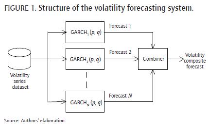
The general structure of the proposed system is presented in the Figure 1. It is composed of N GARCH(p, q) models with the same structure but with different parameter values; all GARCH(p, q) models are fitted using the same sample of data, but using different optimizations with the aim of capturing different features of the volatility dynamics. Each model is used to produce an individual forecast using the available information; finally, all individual forecasts are combined to obtain a volatility composite forecast.

Alternative parameter estimation procedure for the GARCH model

Tsay (2010) presents an alternative estimation procedure based on the minimization of a function of the difference between the volatility and its forecasting. By defining , the GARCH model presented in Eq. (1) would be written out as:

Thus, the previous equation has the same structure of an aRma model where the first expression inside parenthesis corresponds to the autoregressive component while the second correspond to the moving average component. As a consequence, the parameters in the model presented in eq. (3) would be estimated by the following minimization:

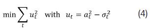
Note that maximize the eq. (2) is not the same thing that the expression in eq. (4) and the optimal parameters in each case are different. As indicated by tsay (2010), the theoretical implications and the practical merits of this approach are unknown and it is necessary further research.

Estimation of the parameters of the garcH model using different error functions

The use of eq. (2) for estimating the optimal values of the parameters in a GARCH(p, q) is based on the assumption of normality of the standardized residuals ε_t; in this sense, when the log-likelihood function is higher, then the probability distribution of εt is nearer to a theoretical standard normal distribution; however, it does not mean that the parameters are optimal in terms of the volatility forecast accuracy.

The estimation procedure proposed by tsay (2010) is focused in the forecast accuracy by minimizing a function of the forecast error; this is, the parameters of the model defined in eq. (3) are estimated executing the minimization presented in eq. (4). However, the parameters of each GARCH(p, q) model would be estimated by minimizing any general loss function.

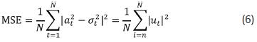
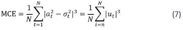
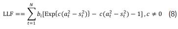
Below, we present a list of commonly employed loss functions on volatility forecast evaluation (Gooijer & Hyndman, 2006; Patton, 2011; Dunis & Huang, 2002). These functions are not robust to noise (Patton, 2011), such that, the optimal forecast is not the true conditional variance. However, we use these functions for fitting the GARCH(p, q) models of our system because of they are able to capture other statistical features of time series that are ignored when the GARCH model is estimated by maximizing the likelihood function; as a consequence, we expect to improve our forecast accuracy respect the classical approach. The functions are a measure that gives us a basis to compare our volatility forecasts with the realized volatility. Under the assumptions for the conditional distribution of daily returns given in Patton (2011), the mse loss function generates an optimal forecast equal to the conditional variance, and thus satisfies the necessary condition for robustness. In addition, we include the linex loss function [proposed by varian (1974) and used by Zellner (1986) and Christoffersen and diebold (1994)] for modeling the possible existence of asymmetries in the response of volatility to the sign of shocks; in practical terms, this means that the model is able to model in a different way large positive and negative differences between squared shocks and variances; in eq. (8), the parameter c controls the asymmetry level, and in most simple case.

• Mean absolute deviation:

• Mean squared error:

• Mean cubic error:

• Linex loss function:

Forecasts combiner

By analyzing the most relevant literature about ensemble averaging methods and forecasts combination techniques, we select the following techniques for combining the volatility forecasts, with ƒ_i, i = 1, ...n, of the GARCH(p, q) models:

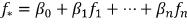
• Simple arithmetical average:

• Combination by multiple linear regression:
where β_i are the parameters.

• Nonlinear optimal combination by using an artificial neural network. In this research, we use the model proposed by Hu and Tsoukalas (1999), where the forecast is obtained as:

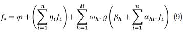
Where φ, β_h, η_h, ω_h, and α_hi are the parameters. g(.) is the sigmoid transfer function:

Note that, the ANN model described by eq. (9) is the combination of a linear regression model and a multilayer perceptron neural network; this allows to the neural network to capture in a better way the linear and nonlinear dynamics in the data. Finally, the model in eq. (9) has nH + 2H + n + 1 parameters to be estimated.

Numerical experiment

Data and preliminary analysis

For our experiment, we use the monthly excess stock returns of the S&P500 index from January of 1926 to December of 1991; see Figure 1. The dataset contains 792 observations and it is commonly used as a benchmark for exemplifying and testing volatility models; see Tsay (2010) and Verhoeven et al. (2002).

Tsay (2010) analyses this time series using all available information (the 792 observations). First, an AR(3)- GARCH(1,1) is postulated for representing the dynamics of the data; the parameters of this model are estimated by maximizing Eq. ((2). Following, all non-significant parameters are dropped and the model is reduced to a GARCH(1,1). The final model proposed by Tsay (2010, page. 136) would be written out as:

Experimental setup

In our numerical experiment, we use the first 708 observations for estimating the parameters of all GARCH(1,1) models and the remaining 84 observations for forecasting. Forecast accuracy, for the fitting and forecasting samples, is measured using the mean absolute deviate (MAD ) and the mean squared error (MSE ) previously defined in Eq. (5) and Eq. (6) respectively.

The setup of our experiment is described by the following steps:

• The GARCH model in Eq. (11) is fitted using the first 708 observations by maximizing the natural logarithm of likelihood function in Eq. (2).

• We rewrite the GARCH(1, 1) model in Eq. (11) as:

And then, we estimate a set of optimal parameters {k,(α1+β1), β1} when each one of the loss functions in Eq. (5), Eq. (6), Eq. (7) and Eq. (8) are minimized. Thus, we obtain four sets of parameters for the model presented in Eq. (12).

• For each GARCH model considered in this experiment, we forecast the volatility one month ahead for both the fitting and the forecasting samples.

• Combined forecasts are calculated using the individual forecasts obtained from the models estimated in steps 1 and 2 as follows:

◊ The simple arithmetical average of the forecasts of each GARCH model.

◊ By using a multiple linear regression.

◊ By using ANN models with H = 1, ..., 4 and n = 5. See Eq. (9). ƒ₁, ƒ₂, ƒ₃, ƒ₄ and ƒ₅ are the forecasts of the models estimated in the steps 1 and 2 by maximizing Eq. (2) and minimizing the MAD, MSE, MCE and LL F(c = 0.038) error functions respectively. Each ANN model is trained fifty times with random initial weights. We prefer the ANN model with the set of parameters minimizing the MSE for the fitting sample.

• The fitting and forecasting mse and mad are calculated. The obtained results, multiplying the mse by 10⁴ and the mad by 10², are presented in tables 2, 3, 4 and 5.

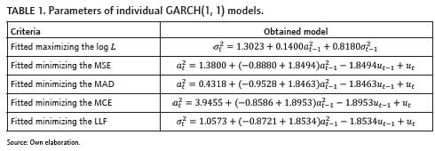
In table 1, the set of parameters for the estimate models maximizing eq. (2) and minimizing eq. (5), eq. (6), eq. (7) and eq. (8) are presented. It is interesting to note that the parameters of models in table 1, do not satisfy the statistical constraints for guaranty positive values of σ_t², but, this is not a problem because of the models are used for forecasting in normal conditions of the market and it is very improbable to obtain negative values for σ_t². In addition, very large values for α_t² occur in abnormal conditions as crashes and bubbles, and it is impossible to forecast such events with any model. Finally, statistical restrictions are not absolute and necessary for obtaining good forecasting models.

In all cases, we use the mse as the evaluation criteria for testing the volatility forecast accuracy (tsangari, 2007; Lopez, 2001), where small values of mse indicate good forecasting accuracy. Additionally, as it is shown in Patton (2011), the mse error function is unbiased and it satisfies the necessary condition for a loss function to be robust to noise in the volatility proxy.

For this work, we implement a prototype in microsoft excel and R program. The optimal parameters of the experts and artificial neural networks were obtained using the solver complement and evolutionary algorithms.

Forecast accuracy of the individual models

We compare and measure the performance of the models using two criteria: the mean squared error (mse), and the mean absolute deviation (mad). In table 2, we present the mse (mad) values for the fitting and forecasting samples when the five individual models are considered. The M₂ model (GARCH fitted by minimizing the mse) results, present the lower value for mse in both samples among all five models. But the mad values for fitting and forecasting samples are not as good. The standard M₁ model (GARCH fitted by maximizing the log l) is overcome by the M₂ model in mse values, and by the M₃ model (GARCH fitted by minimizing the mad) in mad values; this can happen because of the criterion of optimization of these models. The M₅ model (GARCH fitted by minimizing the llF) results show good mse values in comparison with the M₃ model but not in mad values. In this way we look for a model which conforms to our expectation of reaching a balance for the mse (mad) values across both fitting and forecasting samples.

Forecast accuracy of the combined forecasts obtained using a simple average

In table 3, we present the values of the mse and mad statistics calculated for the fitting and forecasting samples. In this case, we consider the average of the all combinations obtained by considering two, three, four and five models. By inspecting the table 3, we found that the M26 model (the average of the forecasts from M₂ and M₃ models) results present the lower mse for the forecasting sample in comparison with the competing models and individual models, but in fitting sample it does not hold for the mse value; the M26 model has the lower mad values. Also, we observe that M₁₉ model (the average of the forecasts from M2, M3 and M5 models) has a mse value near to the mse of M26 model for the forecasting sample and it has low mse value for the training sample.

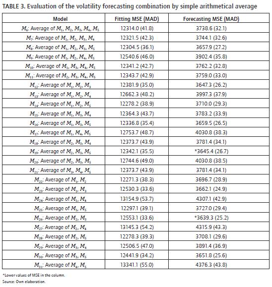
A common practice in forecast combining literature is considering the average of the forecast values of the all available models; in our case, this corresponds to consider the M₆ model in table 3. Reported results show that this model only is better than the M3, M4 and M5 models.

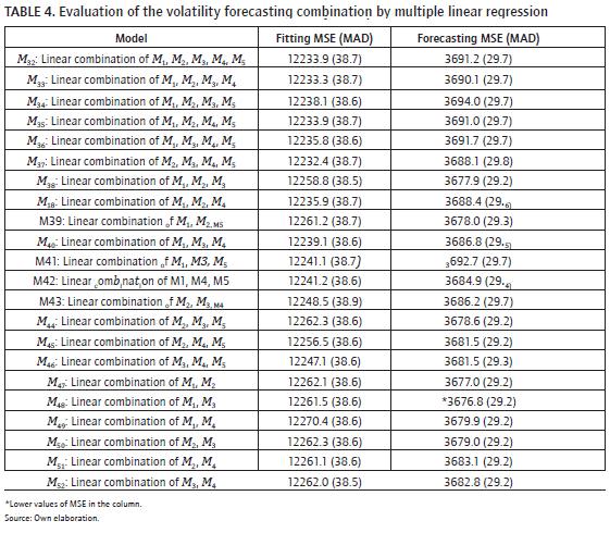
Forecast accuracy of the combined forecasts obtained using a multiple linear regression

In this case we consider the most of the possible linear combinations of individual forecasts. The estimation of the weights was doing by minimizing mse and the obtained results are in table 4. The better linear regression model, with respect to mse value in the forecast sample, is the model that combines forecasts from models M1 and M3, the obtained mse value is 3676.8, which is lower than mse value in the combination by ann with three nodes and the same forecasts; also we observe that simple arithmetical average gets a low mse value of 3662.1 in forecasting sample with the same forecasts. We compare the accuracy between M₄₈ model and individual forecasts from models M1 and M3, the linear multiple regression of these forecasts ( model) is better because it has less mse value than the individuals.

Accuracy of individual forecasts combined using an artificial neural network

In this case, we consider most of the possible combinations of the individual forecasts using the artificial neural network described by equations (9) and (10). For each set of possible inputs, ann models with H = 1, ..., 4 were considered.

In table 5, we present the values of the mse and mad statistics for the fitting and forecasting samples. Several conclusions arise from this table:

• All the considered models have fitting mse values lower than each individual model in table 2. Thus, we conclude that each individual forecaster is able to capture valuable nonlinear information about the volatility dynamics.
• For almost all possible combinations of inputs, in terms of forecast mse values the optimal configuration of the artificial neural network has two neurons in the hidden layer (H = 2).
• The nonlinear combination of individual models is better than each individual model; this is in concordance with the reported experiences in the literature where the composite forecast is more accurate than each individual forecast.
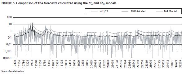
• The M86 model is the preferred among all possible combinations by ann of volatility forecasts because it has a balance for the mse (mad) values across the fitting and forecasting samples in comparison with the individual models. In this case, the composite forecast is obtained by the non-linear combination of the forecasts calculated with the M₂, M₃ and M₄ models (which parameters are calculated by minimizing different loss functions). In Figure 1, we plot the squared shocks for the sample and the forecasts from the M₈₆ model; in Figures 2, 3 and 4, we compare the forecasts of the M86 model with the forecasts of the M₄, M₃ and M₄ models; in these figures are evident that each model captures a different behavior of the squared shocks: the M₂ model, that is estimated by minimizing the mse, (see Figure 2) presents a similar behavior with the M86 model, but the model M₈₆ is able to approximate better the regions with high values of the squared shocks. The model M3, estimated by minimizing the mad, is able to capture better the lower values of the squared shocks. Finally, the model M4 is better for approximating the higher values of the squared shocks. Consequently, the artificial neural network is able to integrate the behavior of each considered individual model and to produce a more accurate forecast.
• The M₅₄, M₅₈ and M₆₄ models results, also present a good and balanced mse (mad) values in fitting and forecasting samples.

Performance of the preferred model

As we indicated in last section, the M86 model is the preferred among all possible combinations by ann of volatility forecasts, in this section we implement a statistical test to show the difference in accuracy between the preferred model and the standard GARCH model (M₁). We also present an evaluation of the preferred model and the standard GARCH model using value at Risk evaluation.

Statistical test of predictive accuracy

A demonstration of the effectiveness of the M86 model over the M₁ model is shown in a statistical test. A test of the null hypotheses of no difference in accuracy between M1 and the preferred model is attempted. We implement the test due to diebold and mariano (1995), which uses the morgan-Granger-newbold statistic for testing of these hypotheses. The test consists in consider the punctual forecasting errors e_1t and e_2t given by two forecasting models, respectively. The used statistic has a Student's t-distribution with T − 1 degrees of freedom. The t statistic is defined by:

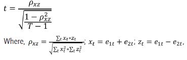
To T; and T is the number of observations.

The morgan-Granger-newbold test results show that the null hypothesis of equal predictive accuracy is rejected between M₁ and M₈₆ models, at 93% level in training sample with a ρ–value of 7,06694×10⁻⁵⁴ and in the forecast sample with a ρ–value of 0,0663.

Value at Risk evaluation

In addition, we have compared the GARCH model fitted by maximizing the log l and the preferred model with respect to the value at risk performance (vaR) for the data. The vaR is defined as the maximum potential loss of a portfolio that occurs under normal market conditions with a predefined probability. Assuming that the returns are normally distributed, the 95%-vaR is computed as 95% quantile of the returns distribution:

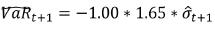
Where is the forecast of the standard deviation given all information until time t.

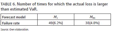
To evaluate the performance of the 95%-vaR estimators we are using the failure rate criterion. The failure rate (F) is the number of times for which the actual loss is larger than the estimated vaR. This criterion is defined as

Where the Dt dummy variable is one if the actual loss is larger than the estimated vaR and zero in other case.

We have used the vaR to evaluate the performance, the failure rate of the M86 model is 4.8% and it is low than the failure rate of the M₁ model (6.2%). We concluded that the model obtained from the combination with an ann can improve the predictive accuracy. The results are shown in table 6.

Conclusions

This work considers the forecasting combination as an alternative to reduce the forecast error of the volatility of the monthly excess returns of s&P500. Several GARCH(1,1) models were estimate, by considering different error mea-sures, and combined by the use of simple arithmetical average and anns to produce a new model that integrate all information from individual models. The results have been showed this forecasting combination approach has a good ability for predict with major accuracy the volatility in comparison with the traditional forecast models.

As future work, several research addresses emerge. First, consider several datasets with different frequencies and proceeding from different markets. Second, analyze other alternative models for specifying the experts in the model. And third, test and justify the use of other types of loss functions for optimizing the parameters of the models used as experts.

References

Amendola, A., Storti, G. (2008). A Gmm procedure for combining volatility forecasts. Computational Statistics & Data Analysis, 52, 3047-3060.         [ Links ]

Andersen, T., Bollerslev, T., Christoffersen, P., Diebold, F. (2005a). Volatility forecasting. PIER Working, Paper no. 05-011.         [ Links ]

Andersen, T., Bollerslev, T., Christoffersen, P., Diebold, F. (2006). Volatility and correlation forecasting. In: Elliott, G., Granger, C.W.J., Timmermann, A. (eds.), Handbook of economic Forecasting. Amsterdam: North Holland Press.         [ Links ]

Bollerslev T. (1986). Generalized autoregressive conditional heteroskedasticity. Journal of Econometrics. 31, 307-327.         [ Links ]

Bollerslev, T., Engle, R.F. (1993). Common persistence in conditional variances, Econometrica, 61, 167-186.         [ Links ]

Brooks, C., Persand, G. (2003). Volatility forecasting for risk management. Journal of Forecasting, 22(1), 1-22.         [ Links ]

Chan, F., & Mcaleer, M. (2003). Estimating smooth transition autoregressive models with GARCH errors in the presence of extreme observations and outliers. Applied Financial Economics, 13(8), 581-592.         [ Links ]

Christoffersen, P. F., & Diebold, F. X. (1994). Optimal Prediction Under Asymmetric Loss (Working Paper no. 167). National Bureau of economic Research.         [ Links ]

Clemen, R. (1989). Combining forecasts: a review and annotated bibliography. International Journal of Forecasting, 5, 559-583.         [ Links ]

Clemen, R., Winkler, R. (1986). Combining economic forecasts. Journal of Business and Economic Statistics, 4, 369-391.         [ Links ]

Diebold, F. X., & Mariano, R. S. (1995). Comparing Predictive accuracy. Journal of Business & Economic Statistics, 13(3), 253-263.         [ Links ]

Donaldson, R.G., Kamstra, M. (1997). An artificial neural network-GARCH model for international stock return volatitlity. Journal of Empirical Finance, 4, 17-46.         [ Links ]

Duan, J. (1997). Augmented GARCH(P, Q) process and its diffusion limit. Journal of Econometrics, 79 (1), 97-127.         [ Links ]

Dunis, C. L., Huang, X. (2002). Forecasting and trading currency volatility: an application of recurrent neural regression and model combination. Journal of Forecasting, 13, 317-354.         [ Links ]

Engle, R.F. (1982). Autoregressive conditional heteroskedasticity with estimates of the variance of United Kingdom inflations. Econometrica, 50, 987-1007.         [ Links ]

Engle, R.F., NG, V. (1993). Measuring and testing the impact of news on volatility. Journal of Finance, 48, 1747-1778.         [ Links ]

Franses, P. H., Dijk, D. Van (2006). Non-linear time series models in empirical finance. Cambridge, United Kingdom: Cambridge University Press.         [ Links ]

Glosten, L. R., Jagannathan, R., & Runkle, D. E. (1993). On the Relation between the expected value and the volatility of the nominal excess Return on stocks. Journal of Finance, 48(5), 1779-1801.         [ Links ]

Gooijer, J.G., Hyndman, R.J. (2006). 25 years of time series forecasting. International journal of forecasting, 22, 443-473.         [ Links ]

Granger, C. W. J. (1989). Combining forecasts-twenty years later. Journal of Forecasting, 8, 167- 173.         [ Links ]

Hashem, S. (1997). Optimal linear combinations of neural networks. Neural Networks, 10, 599-614.         [ Links ]

Haykin, S. (1996). Neural Networks: A Comprehensive Study. Ontario Canada: Prentice-Hall,         [ Links ].

Hu, M. Y., C. Tsoukalas. (1999). Combining Conditional volatility Forecasts using neural networks: an application to the ems exchange Rates. Journal of International Financial Markets, Institutions and Money, 9, 407-422.         [ Links ]

Hull, J., White, A. (1987). The pricing of options on assets with stochastic volatilities. Journal of Finance, 42, 281-300.         [ Links ]

Hyndman, R.J., Koehler, A.B. (2006). Another look at measures of forecast accuracy. International Journal of Forecasting, 22, 679-688.         [ Links ]

Klaassen, F. (2002). Improving GARCH volatility forecasts with regimeswitching GARCH. Empirical Economics, 27(2), 363-394.         [ Links ]

Lopez, J. A. (2001). Evaluating the predictive accuracy of volatility models. Journal of Forecasting, 20, 87-109.         [ Links ]

Lundbergh, S., & Teräsvirta, T. (1998). Modelling economic high-frequency time series with STAR-STGARCH models (Working Paper Series in Economics and Finance No. 291).         [ Links ]

Nazifi, M., & Fatahi, S. (2012). Regime switching GARCH models and GARCH Models, in Stock Market of the Developing Countries' (SSRN Scholarly Paper No. ID 1987428). Rochester, NY: Social science Research Network.         [ Links ]

Nelson D.B. (1991). Conditional heteroskedasticity in asset returns: a new approach, Econometrica, 59, 347-370.         [ Links ]

Patton, A.J. (2011). Volatility forecast comparison using imperfect volatility proxies. Journal of Econometrics, 160, 246-256.         [ Links ]

Poon, S.H., Granger, Clive W.J. (2003). Forecasting volatility in financial markets: a review. Journal of economic literature, 61, 478-539.         [ Links ]

Tang, L.B., Tang, L.X., Sheng, H.Y. (2009). Forecasting volatility based on wavelet support vector machine. Expert Systems with Applications, 36, 2901-2909.         [ Links ]

Taylor, J.W. (2004). Volatility forecasting with smooth transition exponential smoothing. International Journal of Forecasting, 20, 273-286.         [ Links ]

Tsangari, H. (2007). An alternative methodology for combining different forecasting models. Journal of Applied Statistics, 34(4), 403-421.         [ Links ]

Tsay, R. (2010). Analysis of financial time series. New Jersey: Hoboken, Wiley.         [ Links ]

Varian, H. R. (1974). A Bayesian approach to real estate assessment. In Studies in Bayesian Econometrics and Statistics in Honor of Leonard J. Savage (pp. 195-208). North-Holland, Amsterdam.         [ Links ]

Verhoeven, P., Pilgram, B., Mcaleer, M & Mees, A. (2002). Non-linear modelling and forecasting of S & P 500 volatility. Mathematics and Computers in Simulation, 59, 233-241.         [ Links ]

Zellner, A. (1986). Bayesian estimation and Prediction Using asymmetric loss Functions. Journal of the American Statistical Association, 81(394), 446-451.         [ Links ]