Fluid Queue Driven by Finite State Markov Processes

Cola de un fluido modulada por un proceso de Markov con finitos estados

V. Arunachalam^a,*
S. Dharmaraja^b

^a Departamento de Estadística, Universidad Nacional de Colombia, Bogotá, Colombia.
^* Autor de correspondencia: varunachalam@unal.edu.co.
^b Department of Mathematics, Indian Institute of Technology Delhi, New Delhi, India.

Recepción: 25-sep-14 Aceptación: 16-oct-14

Abstract

Steady state distribution of the buffer content of a fluid queue modulated by two independent birth and death processes is found using differential equation techniques to solve a system of equations. The inflow rates are determined by a birth and death process with finite state space and the outflow rate from the buffer is determined by the current state of another independent birth and death process with four states, evolving in the background. Combining these two birth and death processes a continuous time Markov chain is obtained. The steady state buffer content distribution for this fluid queue driven driven by a continuous time Markov chain is thus obtained. Finally, we present numerical results to illustrate the feasibility of the proposed model.

Key words: Birth and Death Processes, Continuous Time Markov Chain, Steady State Distribution.

Resumen

La distribución del estado estacionario del contenido de una cola de fluido en un dispositivo modulado por dos procesos independientes de nacimiento y muerte, se encuentra utilizando técnicas diferenciales para resolver un sistema de ecuaciones. Las tasas de flujo de entrada se determinan mediante un proceso de nacimiento y muerte, con espacio de estados finitos y la tasa de flujo de salida del recipiente se determina por el estado actual de otro proceso independiente de nacimiento y muerte con cuatro estados, que evolucionan en el fondo. Mediante la combinación de estos dos procesos de nacimiento y muerte se obtiene una cadena de Markov de tiempo continuo. Se observa que la distribución del estado estacionario del contenido de una cola de fluido se modula por una cadena de Markov en tiempo continuo. Finalmente, se presentan resultados numéricos para ilustrar la viabilidad del modelo propuesto.

Palabras clave: Cadena de Markov de tiempo continuo, Distribución de estados estacionarios, Procesos de nacimiento y muerte.

1. Introduction

The term queuing system is used to indicate a collection of one or more waiting lines along with a server or collection of servers that provide service to these waiting lines. Delays and queuing problems are most common features not only in our daily-life situations such as at a bank or postal office, at a ticketing office, in public transportation or in a traffic jam but also in more technical environments, such as in manufacturing, computer networking and telecommunications. They play an essential role for business process re-engineering purposes in administrative tasks.

In queueing theory, there are numerous applications where the information flow has to be treated as a continuous stream rather than considering its discrete nature. The resulting queuing models are called fluid queues. Fluid queues are closely related to dams. A dam can be modeled as a reservoir, in which water builds up due to rainfall, is temporarily stored, and then released according to some release rule. Consequently, a fluid queue can be viewed as a dam in which work is buffered until enough capacity becomes available. Fluid queues are used to represent systems where some quantity accumulates or is depleted; gradually over time, subject to some random environment. Fluid models are highly used in performance evaluation of telecommunication systems, modern communication networks, ATM's and statistical multiplexers where the aggregate inflow can be viewed as fluid instead of individual customers.

In a fluid queue model a divisible commodity (fluid) arrives at a storage facility where it is stored in a buffer and gradually released. In a standard queueing system we consider, individual customers or jobs arriving at service facility, possibly wait, then receive service and depart. For such models we count the number of customers in the system and describe the experience of individual customers. In contrast a fluid queue model is used in applications where individual customer is so small that they can hardly be distinguished. It is then easier to imagine a continuous stream of work that flows into the system instead of customers. Fluid queues are used to represent systems where some quantity accumulates or is depleted, gradually over time, subject to some random environment. Some examples of such systems are a dam or a reservoir in which water builds up due to rainfall, is temporarily stored and then released according to some release rule, communication networks where data carried by these networks are packaged in many small packets, etc.

For fluid queues models, we study the buffer content at any time t, which is the amount of work in the system, that can be of finite or infinite capacity. The buffer content cannot be negative, so when the buffer content decreases to zero, the buffer content stays zero as long as the net input rate is negative.

A fluid queue driven by a Markov process, is a two-dimensional Markov process, of which the first component, or level, varies according to the second component, the phase, which is the state of a Markov process evolving in the background. Fluid flows into the buffer at a rate which depends on the state of the background Markov process and fluid flows out from the buffer at some rate. In order that a stationary distribution for the buffer exist, the stationary net input rate should be negative.

Steady state and transient analyses for fluid queues driven by Markov process using different techniques have been studied in much detail by various authors ([4], [7], [13], [15], [2]). [4] uses the continued fraction approach to get the exact steady state solution of a fluid queue driven by an M/M/1 queue. The methodology used to achieve the required solutions by is transforming the underlying system of differential equations using Laplace transforms to a system of difference equations leading to a continued fraction.

In [7] uses matrix analytic technique wherein the computation of the steady state distribution is reduced to the analysis of a discrete time, discrete state space quasi-birth-death model. In van Doorn and Scheinhardt [13] present a survey of techniques for analysing the performance of a fluid queue which receives and releases fluid at rates which are determined by the state of a background birth-death process. The buffer is assumed to be infinitely large, but the state space of the modulating birth-death process may be finite or infinite.

Transient analysis has also been discussed by few authors for some specific queuing models such as fluid queues with background process birth death process or input process governed by M/M/1 queue. Virtamo and Norros [15] analyzed a fluid queue driven by an M/M/1 queue and proposed a spectraldecomposition method. The key of the method is to express the generalized eigenvalues explicitly using the Chebyshev polynomials of the second kind.

In [2] Lenin and parthasarathy discuss fluid queues with infinite buffer capacity driven by an M/M/1/N queue. They find analytically the eigen values of the underlying diagonal matrix and hence the steady state distribution function of the buffer occupancy. [8] and [5] presented the transient solution using a direct approach with the help of recurrence relations. In [8] the transient behavior of stochastic fluid flow models in which the input and output rates are controlled by a finite homogeneous Markov process is analyzed. The solution is based on only recurrence relations.

In [5] a fluid queue driven by an infinite-state birth death process (BDP) whose birth and death rates are suggested by a chain sequence is discussed. The stationary solution for the background BDP suggested by a chain sequence does not exist and hence the stationary distribution for fluid queue driven by such BDPs also does not exist. However their transient probabilities yield a simple closed form solution. In [9] Sericola consider a finite buffer fluid queue receiving its input from the output of a Markovian queue with finite or infinite waiting room. The input flow into the fluid queue is thus characterized by a Markov modulated input rate process and for a wide class of such input processes, a procedure for the computation of the stationary buffer content of the fluid queue and the stationary overflow probability is derived based on recurrence relations.

In [10] the exact transient solution of fluid queue driven by M/M/1 queue are found using recurrence relations and continued fraction. In [11] the exact transient solution of fluid queue driven by BDP with infinite state space by first converting the system of differential equations into a system of algebraic equations using Laplace transform. Then the method of continued fractions is used.

In [6] the time-dependent (or transient) solution for a mathematical model of statistical multiplexing is presented. The model consists of N statistically independent and identical sources and each source alternates between the on state and the off state. The double Laplace transform method is used, and the partial differential equation that governs the multiplexer behavior is reduced to the eigenvalue problem of a matrix equation in the Laplace transform domain.

A lot of study has been carried on the steady state analysis of fluid queues driven by infinite state Markov process but the steady state analysis of fluid queues driven by finite state Markov process has not been extensively performed due to complexity of the problem. The reason being that the Chapman -Kolmogorov equations corresponding to a given fluid queue form a system of conservation laws for which no explicit or closed form solution is available. This motivates to analyse the steady state behaviour. Further, it motivates to obtain various performance measures. In this paper, we present the steady state distribution of the buffer content of a fluid queue modulated by two independent birth death processes is found using differential equation techniques to solve a system of equations [1].

The rest of the paper is organized as follows. Section 2 gives the complete description of the fluid model. Section 3 presents the steady-state distribution of the buffer occupancy. Further, the numerical result is illustrated. Finally, Section 4 concludes the paper.

2. Model Description

Let X := {X(t),t ≥ 0} be a continuous-time stochastic process such that for any t ≥ 0, X(t) is the amount of work offered to the system in the interval [0,t]. The buffer can be interpreted as a fluid reservoir, to which input is offered according to the input process X. The buffer is drained at a constant rate r, i.e., a tap at the bottom of the fluid reservoir releases fluid at rate r as long as the buffer is nonempty. After the fluid is processed, it immediately leaves the system. We write C(t) for the amount of work in the buffer at epoch t, and call this the buffer content.

We describe the fluid queue driven by finite state Markov process. Let {X(t),t ≥ 0} denote the background birth death process which takes values in S = {0,1,2,...,N}. Let λ_i and µ_i represent the birth and death rates respectively. When the system is in state i, the buffer content changes at a rate r_i (which can be both positive and negative). If the buffer is empty, and the Markov process is in a state i with r_i < 0, then the buffer remains empty. We let

The stationary state probabilities p_i, of the background birth death process can then be represented as

In order that a limit distribution for C(t), the content of the reservoir at time t, exist, the stationary net input rate should be negative, that is,

We assume that the above condition is satisfied. In what follows we let

Letting

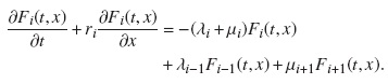
The Kolmogorov equations for the two dimensional process {X(t),C(t)} are given by, for i ∈ S :

But assuming that the process is in equilibrium, we may set Fi(t,x) = Fi(x) and and, hence obtain the system

satisfying the conditions,

The above equations are then solved to get the steady state solution.

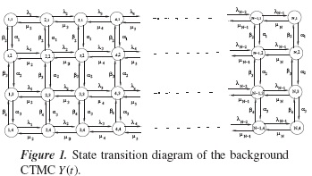
The inflow rates of fluid to the buffer varies with time. The inflow rate is determined by a birth death process (BDP) {X(t), t ≥ 0} with finite state space {1, 2,..., N}. Let λ_i, i = 1, 2,..., N − 1 be the birth rates and µ_i, i = 2, 3,..., N be the death rates of this BDP. When X(t) is in some state i,i ∈{1, 2,..., N}, then the inflow rate into the fluid buffer is given by c_i, which can take any real value (+ve or -ve). When the buffer level reaches zero and the inflow rate at that time is negative, then the buffer level remains at zero until the inflow rate becomes positive. The rates c'_i s, i = {1,2,...,N} represents the random arrival rates of the information at any intermediate node.

The outflow rate from the buffer is determined by the states of another independent BDP {Y(t), t ≥ 0} with four states, 1, 2, 3 and 4. Let α_i, i = 1, 2, 3 be the birth rates and β_i, i = 2, 3, 4 be the death rates of this BDP. When Y(t) is in some state i,i ∈{1, 2, 3, 4}, then the outflow rate from the fluid buffer is given by h_i. Note that h₁ > h₂ > h₃ > h₄. The transitions of {Y(t), t ≥ 0} from one state to another represents the switching of the transmission rates from one step higher to one step lower or vice versa.

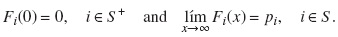
By combining these two above mentioned independent BDPs, we obtain a CTMC with finite number of states. We denote this CTMC by {Z(t), t ≥ 0} with state space S = {(1,1),(1,2),(1,3), (1,4), (2,1), (2,2), (2,3), (2,4),..., (N,1), (N,2), (N,3), (N,4)}. This CTMC has 4N states. The state transition diagram for this process {Z(t), t ≥ 0} is shown in Figure 1. Note that, in this CTMC, we have assumed that diagonal transitions are not feasible in a small time interval. Whenever, Z(t) = (i, j), i ∈ {1, 2,..., N}, j ∈{1, 2, 3, 4}, the outflow rate from the buffer is h_j. The considered fluid model driven by the underlying CTMC with four different outflow rates and state dependent inflow rates is shown in Figure 2.

3. Buffer Occupancy Distribution

In this section, we obtain the steady-state distribution of the buffer occupancy. First, we describe the background stochastic process. Next, we describe the governing equation for the fluid model. Let

p_{i, j}(t) = Pr [The state of the CTMC {Z(t), t ≥ 0} is (i,j) at the time t],

For simplification, we enumerate the state (i, j) under a single index. Let q₁(t), q₂(t),..., q₄N−1(t),q₄N (t) be the 4N state probabilities of the CTMC {Z(t), t ≥ 0} which are given by:

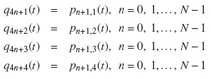
Hence, corresponding to the new indexing of the states of {Z(t), t ≥ 0}, we define a new CTMC, {K(t), t = 0} with finite state space S = {1, 2, . . . , 4N}. The state transition diagram for this process {K(t), t ≥ 0} is shown in Figure 3.

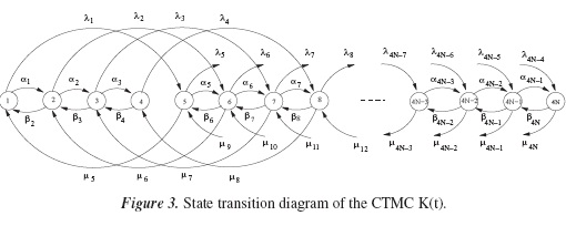
Now, as a consequence, the buffer content of the considered fluid queue is now determined by the CTMC {K(t), t ≥ 0}. The generator matrix of the CTMC {K(t), t ≥ 0}, Q is given by

The buffer content at any time t is denoted by C(t) and we assume that C(0) = 0. Hence, we now have a bi-dimensional stochastic process {C(t), K(t), t ≥ 0}. The net flow rate into the buffer, denoted by r_i, is given by

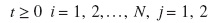
For n = 0, 1, 2, ... , N -1; j = n+1

We have the following differential equation [14]:

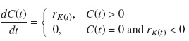
This implies that whenever the CTMC {K(t), t ≥ 0} is in state i, i ∈ S , the corresponding net flow rate is r_i. And each r_i must be either positive or negative with at least one r_i > 0 because otherwise the buffer will remain empty forever.

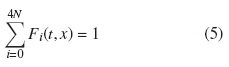
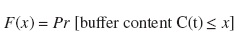
The buffer occupancy distribution is defined as

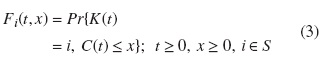
where F_i(t,x) is the probability that the background Markov process {K(t), t ≥ 0} is in some state i and the buffer content is less then or equal to some quantity x. The distribution of the buffer occupancy is a mixed distribution with a positive mass at x = 0, given as

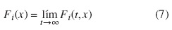
And in the long run, as t →∞ and x →∞,

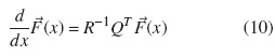
The governing differential equation for the fluid queue is given by [12]

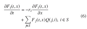
where F_i(t, x) is defined in equation (3) and Q is given in equation (1).

In the next subsection, we obtain the steady-state distribution for the buffer occupancy.

We define the steady-state distribution (in the long run as t →∞) as

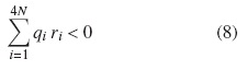
where F_i(t,x) is defined in equation (3). For the steady-state solution to exist, we need a stability condition. For the fluid queue, this stability condition is that as t →∞, the stationary net flow rate should be negative, that is

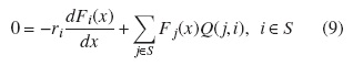
Now, using (7), in the long run as t →∞, equation (6) becomes

Let be column vector formed by the 4N stationary probabilities and is given by

and let R be the diagonal matrix given by

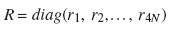
Hence, the equation (9) in matrix form is given by

Theorem 1. The steady-state distribution of buffer occupancy is given by

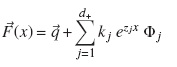
where 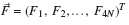and is the column vector of steady-state probabilities of the CTMC {K(t), t ≥ 0} model. That is, = (q₁, q₂,..., q_4N)^T and z₁, z₂,..., z_4N are the 4N eigen values of R⁻¹Q^T with respective eigen vectors Φ₁, Φ₂,..., Φ_4N. d⁺ is the number of states of the CTMC {K(t), t ≥ 0} with positive net flow rate and k ^′ _js are some constants.

Please refer [3, 11] for the proof.

Now, we present the numerical results obtained for the steady-state distribution of the buffer occupancy. For the purpose of numerical illustration, we have taken the number of states, 4N = 24. The values of other parameters are given in Table 1.

Now, we present the steady-state distribution of the buffer occupancy. The steady-state distribution of buffer occupancy is defined as

Hence, we have

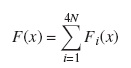
where F_i(x), i ∈ S are obtained by using Theorem 1.

Figure 4 shows the variation of F(x) with the buffer content x, where x is varied from 0 to 10000.

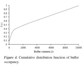
It is observed that there is a positive mass at x = 0 and F(x) → 1 as x →∞. Hence, this shows that the buffer occupancy has mixed distribution.

4. Conclusion and Future Work

Most of the work done in the fluid queues involve a single BDP as the background Markov process. But, we present a fluid queue which is driven by two independent background BDPs, which in turn give rise to a CTMC. Using the fluid model, the steadystate distribution of the buffer content is obtained. As future work, we are planning to obtain the transient distribution of the buffer content using fluid queue approach.

Acknowledgements

S. Dharmaraja would like to thank Universidad Pedagógica y Tecnológica de Colombia Tunja, Colombia for supporting visit during the month of June 2013.

References

[1] V. Arunachalam, V. Gupta and S. Dharmaraja, "A fluid queue modulated by two independent birth-death processes". Computers and Mathematics with Applications, vol. 60, pp. 2433-2444, 2010.         [ Links ]

[2] R. B. Lenin and P. R. Parthsarathy, "A computational approach for fluid queues driven by truncated birth-death processes", Methodology and Computing in Applied Probability, vol. 2, pp. 373-392, 2000.         [ Links ]

[3] D. Mitra, "Stochastic theory of a fluid model of producers and consumers coupled by a buffer", Advanced Applied Probability, vol. 20, pp. 646-676, 1988.         [ Links ]

[4] P. R. Parthsarathy, K.V. Vijayashree and R.B. Lenin, "An M/M/1 driven fluid queue continued fraction approach", Queuing Syst. Theory Appl., vol. 42, pp. 189-199, 2002.         [ Links ]

[5] P. R. Parthsarathy, B. Sericola and K.V. Vijayashree, "Transient analysis of a fluid queue driven by a birth and death process suggested by a chain sequence", Journal of Applied Mathematics and Stochastic Analysis, pp. 143-158, 2005.         [ Links ]

[6] Q. Ren and H. Kobayashi, "Transient solutions for the buffer behaviour in statistical multiplexing", Performance Evaluation, vol. 23, pp. 65-87, 1995.         [ Links ]

[7] V. Ramaswami, Matrix analytic methods for stochastic fluid flows, In D. Smith and P. Hey, Editors, Teletraffic Engineering in a Competitive World (Proceedings of the 16th International Teletraffic Congress), Elsevier Science B.V., Edinburgh, UK, pp. 1019-1030, 1999.         [ Links ]

[8] B. Sericola, "Transient analysis of stochastic fluid models", Performance Evaluation, vol. 32, pp. 245-263, 1998.         [ Links ]

[9] B. Sericola, "A Finite Buffer Fluid Queue Driven by a Markovian Queue", IRISA-INRIA, Queueing Systems, vol. 38, 213-220, 2001.         [ Links ]

[10] B. Sericola, P.R. Parthasarathy and K.V. Vijayashree, "Exact transient solution of M/M/1 driven fluid queue", International Journal of Computer Mathematics, vol. 82, no. 6, pp. 659-671, 2005.         [ Links ]

[11] T. E. Stern and A. I. Elwalid, "Analysis of separable Markov-modulated rate models for information-handling systems", Advanced Applied Probability, vol. 23, pp. 105-139, 1191.         [ Links ]

[12] E. A. van Doorn, A. A. Jagers and J. S. J. de Wit, "A fluid reservoir regulated by a birthdeath process", Stochastic Models, vol. 4 pp. 457-472, 1988.         [ Links ]

[13] E.A. van Doorn and W. R. W. Scheinhardt, "Analysis of birth-death fluid queues", Proceedings of the Applied Mathematics Workshop, Vol. 5, Korea Advanced Institute of Science and Technology, Taejon, pp. 13-29, 1996.         [ Links ]

[14] E.A. van Doorn and W.R.W. Scheinhardt, A fluid queue driven by an infinite-state birthdeath process, In Proc. 15th International Teletraffic Congress (V. Ramaswami and P. E. Wirth, eds.) Elsevier, Amsterdam, pp. 465-475, 1997.         [ Links ]

[15] J. Virtamo and I. Norros, "Fluid queue driven by an M/M/1 queue", Queuing Syst. Theory Appl., vol. 16 pp. 373-386, 1994.         [ Links ]