


Services on Demand
Journal
Article
 English (pdf)
 Article in xml format
 Article references
 Send this article by e-mail
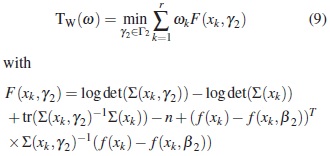
Indicators
-
 Cited by SciELO
 -
 Access statistics
Related links
-
 Cited by Google
 -
 Similars in
SciELO
Similars in
SciELO -
 Similars in Google
Share

 Permalink
Ciencia en Desarrollo
Print version ISSN 0121-7488
Ciencia en Desarrollo vol.7 no.1 Tunja Jan./June 2016
Optimal Population Designs for Discrimination Between Two Nested Nonlinear Mixed Effects Models
Diseños poblacionales óptimos para discriminación entre dos modelos no lineales de efectos mixtos anidados
M. E. Castañeda L.a,*
V. I. López-Ríosb
a Universidad de Antioquia, Medellín, Colombia.
* Autor de correspondencia: maria.castaneda@udea.edu.co.
b Profesor asociado, Escuela de Estadística, Universidad Nacional de Colombia, Medellín, Colombia.
Recepción: 21-sep-2015 Aceptación: 20-ene-2016
Abstract
In this paper we consider the problem of finding optimal population designs for discrimination between two nested nonlinear mixed effects models which differ in their intra-individual covariance matrix. The criterion proposed is a generalization of the T-optimality criterion. For this criterion an equivalence theorem is provided. The application of the criterion is illustrated with an example in pharmacokinetic.
Key words: Optimal Designs, Mixed Effects Model, T-Optimal Designs.
Resumen
En este artículo se considera el problema de encontrar diseños poblacionales óptimos para dicriminar entre dos modelos no lineales de efectos mixtos anidados, los cuales difieren en su matriz de covarianza intraindividual. El criterio propuesto es una generalización del criterio de T-optimalidad; para él se proporciona el respectivo teorema de equivalencia, y su aplicación se ilustra por medio de un ejemplo en farmacocinética.
Palabras clave: diseños T-óptimos, diseños óptimos, modelo de efectos mixtos.
1 Introduction
In the application of optimal design theory one of the basic assumptions is to assume that the model used to describe a given phenomenon or process is the correct model. However, in the practice there may exist several candidate models. One way of to select the most adequate model among several candidates is conducting an experiment designed so that the observations obtained allow us to discriminate between the models in the best way possible. This leads to the problem of to find the optimal experimental conditions using some optimality criterion for discriminate between competing models.
In the case of fixed effects models a commonly used criterion for discriminating between two competing homoscedastic models is the T-optimality criterion, which was proposed by [1]. Under normally distributed observations, the T-optimal design provides the most powerful F-test for the lack of fit of one model when the other is assumed to be true. The criterion has been generalized for other fixed effects models see [18, 19].
The nonlinear mixed effects models are particularly useful in longitudinal studies such as population pharmacokinetics experiments, assay analysis and studies of growth, in which a limited number of samples can be obtained from each individual. These models distinguish two classes of variation: the random variation among observations within a given individual (intra-individual) and random variation among individuals (inter-individual) [3, 4]. This separation of variability allows the estimation of population characteristics from sparse samples per individual in a set of subjects without requiring individual estimation of the parameters. Depending of the application and nature of data, different covariance structures may be considered to model the two class of variation. For example, in some situations it is common practice not to assume a particular structure for the inter-individual variation, whereas for intra-individual variation can be considered different structures, among them, the usual structure which assume independent observations with constant variance, compound symmetry and autoregressive structures, constant coefficient variation structure, variance function which depends on the conditional mean response, or combinations of these structures [7, 21, 12]. Under a nonlinear mixed effects model, a population design is defined by the number of individuals to study and the individual designs to be performed in the individuals (number of samples and the sampling times) [11]. Thus, assuming that the response function and the inter-individual covariance model have been correctly specified, it may be of interest the problem of designing an experiment in a group of individuals with sparse samples per individual for discrimination between two competing intra-individual covariance models which may be nested.
Although some approaches such as those described below have been proposed for discriminate between two nonlinear mixed effects models, these may be inappropriate or less efficient in situations involving nested models as the previously considered. Waterhouse et al. in [22] proposed the product D-optimality criterion based on the product of the determinants of the Fisher information matrices for to find designs useful for both parameter estimation and model discrimination. For nonlinear models, such designs may be less efficient for discriminate that the T-optimal designs. Vajjah and Duffull in [20] proposed a robust T-optimal design method which does not depend on a priori selection of the true model. However, in the particular case of two nested intra-individual variation models this methodology can be not applied because the T-optimal designs are based only on the fixed effects models without residual error. Kuczewski et al. in [9] proposed an extension of the T-optimality criterion for heteroscedastic models, for discriminate between two multiresponse models. The criterion is derived in the case of non-nested models and can be applied directly when all individuals are observed under the same experimental conditions. Therefore, alternative methods for discrimination in the case of nested models are required. In this work, we consider the problem of to find optimal population designs for discrimination between two nested nonlinear mixedeffects models which differ in their intra-individual covariance matrix. We propose a generalization of the T-optimality criterion for this case. Our approach can be applied to population studies for groups of individuals with different sampling scheme where each sampling scheme is a multidimensional point in a finite space of admissible sampling sequences.
This paper is organized as follows. In Section 2 we present the nonlinear mixed effects model considered in this work, optimal design concepts and the model discrimination problem. In Section 3 a generalization of T-optimality criterion is defined and a necessary and sufficient condition for optimality of a design is given. In the section 4 we present an example where the criterion is applied to discriminate between two pharmacokinetic models. Finally, some conclusions and further work are given.
2 Theoretical Background
2.1 Nonlinear Mixed Effects Model
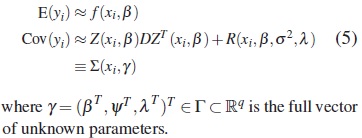
We assume that for each individual i in a population of N individuals the number of different observations available is n. Let yi = (yi1,..., yin)T be the vector of repeated measurements for the ith individual and xi = (xi1,..., xin)T the n × 1 vector of sampling times where xij belongs to a finite set  consisting of t different measurement times. It is assumed that the measurements made on different subjects are independent. To model the relationship between yi and xi we consider a nonlinear mixed effects model which may be written as hierarchical two-stage model, see [3]:
Stage 1. Intra-Individual Model
In this stage the variability among observations within a given individual (intra-individual) is modeled.
Suposse that

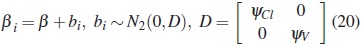
where βi is a (p × 1) vector of parameters for the ith individual; f (xi, βi) is an n × 1 vector function, f (xi, βi) = (f (xi1, βi),..., f (xin, βi))T where f is a known nonlinear function of βi; and εi is the n × 1 random errors vector.
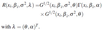
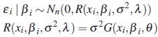
It is assumed that εi|βi ∼ Nn(0, Cov (εi|βi)) with

where R(xi, βi, σ2 ,λ) is an (n × n) matrix and is called the intra-individual covariance matrix, which depends on the parameters σ2 > 0 and λ ∈ Ω ⊂ Rd .
For a given individual, the matrix R takes into account the nature of intra-individual variation and may be choosen in such a way that reflects the heterogeneity of variance, and the correlation among observations, or both. For example, in the case of data from pharmacokinetic experiments and growth studies a common model is
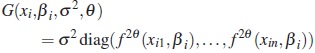
and λ = θ. This matrix corresponds to uncorrelated errors with variance proportional to a power of the conditional mean. If the repeated observations are taken over time, a model for serial correlation can be considered, for example, the autoregressive (AR) model of order one for equally spaced data in time. Thus a model with this correlation structure and constant variance is  and λ = α. Also, we can consider the case where the errors have nonconstant variance with correlation structure by the specification
For others structures of intra-individual correlation see [12].
Stage 2. Inter-Individual Model
In model (1), the variation among individuals (inter-individual) is modeled through the individual specific parameters βi. In order to account the possible dependence of this variation on individual characteristics, a model for βi is provided in this stage.
Suposse that
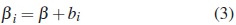
where β is a (p ×1)vector of population parameters and bi is a (p × 1) vector of random effects associated with individual i. It is assumed that the bi are independent and normally distributed with mean 0 and variance-covariance matrix D and that the bi and εi are independent. The matrix D is called the inter-individual covariance matrix. The parameter σ2 and the distinct elements of the covariance matrix D can be arranged in a single vector ψ of covariance parameters.
First-order approximation model
An approximation to the marginal distribution of yi can be derived taking a first-order Taylor series expansion of the model (1) about E(bi)=0. This expansion yields to the linealized model given by
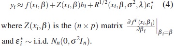
Thus, under (4) the approximate marginal distribution of yi is normal with approximate mean vector and variance-covariance matrix given by
2.2 Population Designs
For the given model, suppose that nk independent observations are taken at point 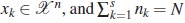 , where s is the number of distinct xk. For example, consider a study in which nk individuals are observed under the conditions vector xk =(xk1,...,xkn), with the total number of individuals N. Then the collection of xk and nk, represented by
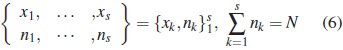
is called population design [11, 6]. The set  is called the design region and the points xk are called design points. We will use the term group to denote the individuals who are allocated to the same sampling sequence xk. The collection
 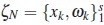 where
where  is called normalized or exact population design with weights vector ω = (ω1,...,ωs). For fixed values of the total number of individuals N and the number of sampling times n, the population optimal design problem consists in to find the design by a choice of distinct values for the sampling times vector x ∈ and values for the number subjects assigned to vector x so that the resulting design maximizes some optimality criterion which will depend on the objective of experiment. The design is said to be optimal with respect to that criterion [5]. The most commonly used optimality criteria usually depend on the unknown model parameter. One approach is to construct locally optimal designs which requires to specify a prior estimate of parameter and then address the optimization problem for this specific value [5] .
Since finding an optimal exact design is a discrete optimization problem which may be difficult from both analytical and computational points of view, the corresponding approximate design should be considered one in which the weights ωk may be any real numbers from the interval [0,1]. Thus, the collection
is called approximate population design. The weight ωk represents the proportion of total individuals that should be observed at the point xk.
If r denotes the number of elements in the design region then the design ζ can be specified by the vector of weights 
Under this representation, if ωk =0 this means that the corresponding design point is not used in the experiment. The set of points xk in the design region for which the design ω has nonzero weights ωk is called the support set of ω and is denoted by supp(ω).
After optimization, the number of individuals in each group is obtained from the optimal weights by using nk =N ×ωk. This can yield noninteger number and therefore a rounding procedure is applied [14].
In what follows, we adopt the approximate locally optimal design approach and we use the approximate design ω =(ω1,...,ωr).
2.3 The Problem of Model Discrimination
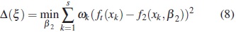
In the case of fixed effects models, these are models that do not contain the level of random effects, one most commonly used criterion for model discrimination is T-optimality proposed by Atkinson and Fedorov in [1]. For two competing homoscedastic models this criterion is based on the assumption of one model ft (x) = f1(x,β1)is the true model. The T-optimal design is a design that maximizes
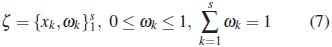
where  such that 0 ≤ ωk ≤ 1 and
  , and f2(x,β2) is the rival model.
If the functions fj(x,β j) depend linearly on the parameter β j, j = 1,2, then the quantity Δ(ξ) is proportional to noncentrality parameter of the χ2 distribution of the residual sum of squares for the second model. The T-optimal design provides the most powerful F test for the lack of fit of the second model when the first is true. For nonlinear models this result is asymptotic.
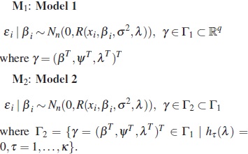
For nonlinear mixed effects models, assuming that the response function f and the inter-individual model are correctly specified, we consider the discrimination problem between two nested intraindividual variation models. Specifically, let R1 and R2 be two alternative models to describe the intra-individual variability. It is assumed that R2 is nested within R1 in sense that both models involve the same structure R(xi,βi,σ2 ,λ) and with respect to the parameter λ the parameter space Ω2 of R2 is a subset of the parameter space Ω1 of R1 defined by the imposition of κ equality constraints. That is, Ω2 = {λ ∈ Ω1 | hτ (λ) = 0,τ = 1,...,κ} where the functions hτ (λ) are assumed to be continuously differentiable.
The objective is to find the appropriate form of the intra-individual covariance matrix R. This can be achieved by performing an experiment designed in such a way that observations obtained allow us to discriminate between R1 and R2 in the best way possible. For to determine such experimental design, we propose an optimality criterion which corresponds to a generalization of the T-optimality criterion. This design provides the most powerful likelihood ratio test when the largest model is assumed to be the true model. In the next section the criterion is derived.
3 Criterion for Discrimination Between Two Intra-Individual Models
The discrimination between two nested intraindividual variation models leads to the discrimination between two nested nonlinear mixed effects models M1 and M2 such that the second stage is as in (3) for both models and the first stage of each model represents a different assumption about intraindividual model, specifically:
M1: Model 1
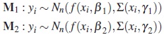
Assuming that the approximation (4) is exact, these models can be represented as:
In order to discriminate between these models, assuming that the largest model is completely known, we propose to find the approximate design ω*that maximizes the following generalization of Toptimality criterion over the set Ξ:
where 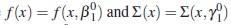 for some known value
  . The design ω* be called Twoptimal, where the letter W refers to the withinindividual variance-covariance matrix. This design is locally optimal because it depends on the values of γ1.
For this class of nonlinear mixed effects models, this criterion may be considered as an extension of proposed criterion by [9] for groups with different designs and a single response.
The justification of criterion is follows.
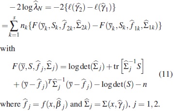
Let γ0 denote the true value but unknown of parameter γ. To discriminate between the alternative models M1 and M2 we consider the likelihood ratio test for the model selection. Since M2 is nested within M1, the testing problem can be formulated as:

where Γ2 = {γ =(βT ,ψT ,λT )T | γ ∈ Γ1, hτ (λ)= 0,τ = 1,...,κ}.
The following assumptions will be required:
(A1) Γ1 is a compact set, (A2) f (x,β) is a continuous and twice continuously differentiable function in Γ1, (A3) Σ (x,γ) is a continuous and twice continuously differentiable function in Γ1.
Let yk1,...,yknk be the independent observations vectors of individuals with sampling times vector xk, k = 1,...,s. Assuming that the approximation (4) is exact, yk1,...,yknk , are Nn( f (xk,β),Σ(xk,γ)) random vectors (k = 1,...,s).
For the testing problem (10), the likelihood function based on the s independent samples is
where  are the maximum likelihood estimators over Γ1 and Γ2 respectively, the likelihood ratio test of H0 against H1, reject H0 for large values of
Under H0, the test statistic  has asymptotically a central χ2 distribution with κ degrees of freedom. Therefore, an approximate test of size α of H0 is to reject H0 if
 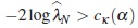 , where cκ (α) denotes the upper 100α% point of the
  distribution.
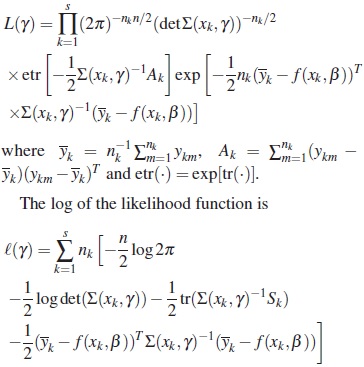
In analysis of mean and covariance structure models, the function  is known as the maximum likelihood discrepancy function which measures the discrepancy between the sample moments and the moments based in the model which depends on the parameter γ (see [16]). The minimizing of this function leads to the maximum likelihood estimator for ith group. Extensions of discrepancy function to more than one group is straightforward [2]. Specifically, the discrepancy function for s groups is defined as
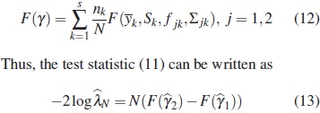
Now, the power of this test, 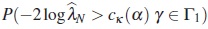 , is a function of the alternative parameter value γ. Given a specific value of N denoted by N0 and a specific alternative parameter value
  close to Γ2, this probability can be approximated by considering the asymptotic distribution of
  under a sequence
  of local alternatives converging to a point
  in Γ2 (see [17]). It is assumed that is an interior point of Γ1. The parameter value is identified then with
  . Since F(γ) in (12) is a discrepancy function, under assumptions (A1)-(A3) and regularity conditions, this asymptotic distribution is the noncentral Chi-square distribution
  with κ degrees of freedom and noncentrality parameter δ, which can be approximated by the value:
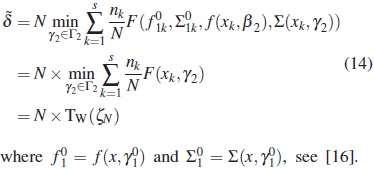
Since the power of test is a monotonically increasing function of the noncentrality parameter, from (14) the power is an increasing function of TW (ζN) and hence can be maximized by the choice of design ζN .
Finally, the exact design ζN can be replaced by the corresponding approximate design ζ which is represented by ω. Thus we obtain the TW-criterion defined in (9).
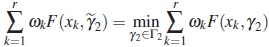
A Necessary and Sufficient Condition for TW-Optimality
The following definition is fundamental for characterizing of Tw-optimal designs.
Definition 1. A design ω is called a regular design if the following set
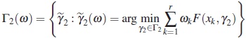
is singleton, otherwise it is called singular design.
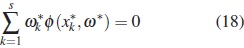
Hence, if ω is a regular design and  , then
  is the unique solution of the equation
The following theorem is the equivalence theorem for Tw-criterion which provides precise conditions for checking whether a particular design is Tw-optimal.
Theorem 1. Let ω* be a regular design. Under the assumptions (A1)-(A3):
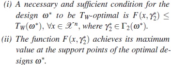
Proof. The proof of this theorem is similar to the proof of Theorem 1 in [9].
(i) First, we prove that the criterion Tw is a concave function. To this end, suposse ω1, ω2 ∈ Ξ and α ∈ [0, 1]. It is clear that Ξ is a convex set. Let ω = (1 − α)ω1 + αω2, then
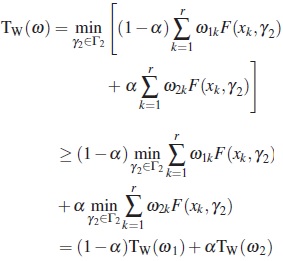
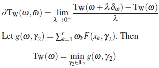
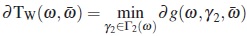
Now, the directional derivative of Tw at ω in the direction of 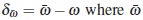 is any design, is given by
Since f (x, β) and Σ (x, γ) are continuous and twice continuously differentiable in Γ1,it follows that 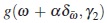 is a continuous function at α and in Γ2. Additionally,
 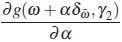 exists and is also continuous at α and in Γ2. Hence, applying the Theorem 3.3 of [13], we get
where  in the direction derivative of g at ω in direction of
 , then
and using the definition of directional derivative
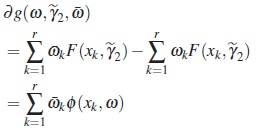
As ω* is a regular Tw-optimal by assumption, we have  and from (15) it fol
where ω is any design.
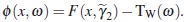
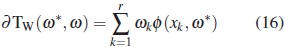
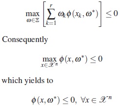
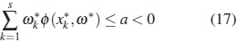
Since Tw(ω)is a concave function of ω, then the plasma concentration as a function of time. The the nonpositivity of the directional derivative simplest compartmental model assumed for such a at ω*is a necessary and sufficient condition relationship is the nonlinear model given by, for the optimality of ω*. From this fact and by (16), it follows that a necessary and sufficient condition for the optimality of ω* is that ω* fulfills the inequality
(ii) We assume the contrary, this mean there is a set 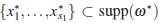 and a scalar a such that
 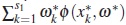 ≤ a < 0 and φ(x * ,ω*)= 0 for x * ∈ supp (ω* )\{x1,...,xs1 }. Then
where s is the number of elements in supp(ω*). From (15) taking  ,wehave
This contradiction proves the assertion.
4 An Example
In this section we present an example to illustrate the use of the criterion proposed. This is a theorical pharmacokinetics example described by [8] in a simulation study and used by [10] in the application of methods to find optimal population designs to estimate population characteristics of the pharmacokinetics of a drug in sparse-sampling experiments. We reproduce the models and parameters values from the second study.
The pharmacokinetic studies seek to understand the process of drug absortion, distribution and elimination using for example kinetic models to describe the plasma concentration as a function of time. The simplest compartmental model assumed for such a relationship is the nonlinear model given by,
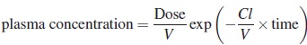
where V is the volume of distribution, CL is the clearance and Cl/V represents the rate of elimination; V and CL are the parameters of model which vary from individual to individual across the population under study. Suposse that the objective is to design an experiment for discriminate between two alternative models for variation within individuals. The model M1 assumes uncorrelated errors with variance proportional to a power of mean response and the model M2 also assumes uncorrelated errors but constant variance. The models are as follows.
The nonlinear mixed effects model can be written as
Stage 1. (Intra-Individual Variation)
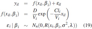
where, for the subject i, yil represents the lth concentration measurement taken at time xil, Cli is the clearance, Vi is the volume of distribution and βi = (Cli, Vi)T. The dose D = 1 is fixed for all individuals.
Stage 2. (Inter-Individual Variation)
where β =(Cl, V )T is the mean values vector.
The two alternative models for the withinindividual covariance matrix R (xi,βi,σ2 ,λ)are:
M1. Variance proportional to a power of mean response and uncorrelated errors
where

M2. Constant variance and uncorrelated errors
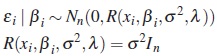
It is assumed that the variance σ2 is a fixed constant equal to 0.15 for both models.
Since the model M2 is nested within M1, the true model is M1 with the population parameter vector given by
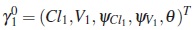
where Cl1 = 0.5, V1 = 0.2, ψCl1 = 0.01, ψV1 = 0.0016 and θ =1.
For the alternative model M2 the population parameter vector is

The set of possible sampling times considered is ={0.05,0.15,0.3, 0.6,1} hours after administration. We assume that three observations are available for each patient, n = 3, without replicates at an identical time point, which in a pharmacokinetic study is a sparse sampling situation. Therefore, the design region is given by the set of combinations of three sampling times from , that is,  containing 10 elements. The sequences are:
x1 =(0.05,0.15,0.3), x2 =(0.05,0.15,0.6),
x3 =(0.05,0.15,1), x4 =(0.05, 0.3,0.6),
x5 =(0.05,0.3, 1), x6 =(0.05, 0.6,1),
x7 =(0.15,0.3, 0.6), x8 =(0.15,0.3, 1),
x9 =(0.15,0.6, 1), x10 =(0.3,0.6, 1).
To find the locally TW-optimal design we used the nominal values of parameters defined previously like the local parameters and the design region  . The optimal design was calculated optimizing the Tw-criterion implemented through an algorithm in R[15]. The function nlminb was used for the optimization in the design region .
The local TW-optimal design obtained is a twopoint design
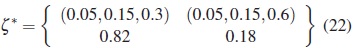
and the parameter vector for the M2 model obtained in the optimization procedure is
Thus, if the objective is to design a new experiment with sparse sampling for discriminate between the M1 and M2 models then for about a 82% of the patients, blood samples should be taken at 0.05, 0.15 and 0.3 hours, and for about 18% blood samples should be taken at 0.05, 0.15 and 0.6 hours.
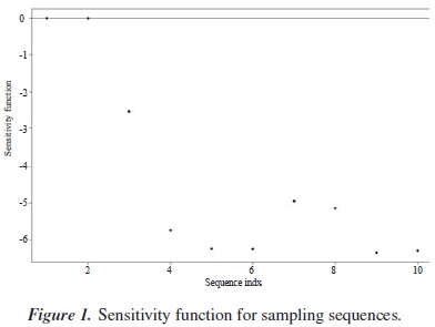
To check that the design obtained is Tw-optimal we use the equivalence theorem. First, we enumerate all candidate sampling sequences, that is, the elements of and calculate the sensitivity function  for each sampling sequence. Then plot the sensitivity function as a function of index i. The resulting plot is shown in Figure 1. From this plot it is clear that the design ζ* consisting of the x1 and x2 sequences is Tw-optimal.
5 Conclusions
A generalization of T-optimality criterion has been proposed for discriminate between two nested nonlinear mixed effects models. The first stage of each model represents a different assumption about intraindividual random variation and the second stage is the same for both models. Assuming that the response function is common for both models and it is correctly specified, we observe that the criterion development in this paper may be considered an extension of the proposed criterion by [9] for groups with different designs and a single response.
In the case of nested models an alternative criterion for discriminate between models is the DS-criterion which is appropiate when interest is in estimating a subset of s parameters. Since the rival models considered in this paper are nested this criterion may be applied. The comparison between the performances of Tw-and DS-optimal designs will be studied in future papers.
Another future work involve the study of designs with multiple objectives as the compound design. For example, the compound criteria for parameter estimation and for discrimination between models using D-optimality with Tw-optimality and Doptimality with DS-optimality.
References
[1] A. C. Atkinson, and V. V. Fedorov, "The design of experiments for discriminating between two rival models", Biometrika, vol. 62, pp. 57-70, 1975. [ Links ]
[2] K. Bollen, "Estructural Equations with Latents Variables", John Wiley & Sons, New York, Inc, 1989. [ Links ]
[3] M. Davidian, and D. M. Giltinan, "Nonlinear Models for Repeated Measurement Data", Chapman & Hall, London, 1995. [ Links ]
[4] E. Demidenko, "Mixed Models: Theory and Applications", John Wiley & Sons Inc, New York, 2004. [ Links ]
[5] V. V. Fedorov, and P. Hackl, "Model-Oriented Design of Experiments", Springer, New York, 1997. [ Links ]
[6] R. Gagnon, and S. Leonov, "Optimal population designs for PK models with serial sampling", Journal of Biopharmaceutical Statistics, vol. 15, pp. 143-163, 2005. [ Links ]
[7] D. Hand, and M. Crowder, "Practical Longitudinal Data Analysis", Chapman & Hall, London, 1996. [ Links ]
[8] Y. Hashimoto, and L. Sheiner, "Designs for population pharmacodynamics: value of pharmacokinetic data and population analysis", Journal of Pharmacokinetics and Biopharmaceutics, vol. 19, pp. 333-353, 1991. [ Links ]
[9] B. Kuczewski, B. Bogacka, and D. Uci´nski, "Optimum designs for discrimination between two nonlinear multivariate dynamic mixedeffects models", Biometrical Letters, vol. 45, pp. 1-28, 2008. [ Links ]
[10] F. Mentré, P. Burtin, Y. Merlé, J. Bree, A. Mallet, and J. Steimer, "Sparse-sampling optimal designs in pharmacokinetics and toxicokinetics", Drug Information Journal, vol. 29, pp. 997-1019, 1995. [ Links ]
[11] F. Mentré, A. Mallet and D. Baccar, "Optimal design in random-effects regression models", Biometrika, vol. 84, pp. 429-442, 1997. [ Links ]
[12] J. C. Pinheiro and D. M. Bates, "Mixed-Effects Models in S and S-PLUS", Springer, New York, 2000. [ Links ]
[13] B. N. Pshenichny, "Necessary Conditions for an Extremum", Marcel Dekker, New York, 1971. [ Links ]
[14] F. Pukelsheim, Optimal Design of Experiments, John Wiley & Sons Inc, New York, 1993. [ Links ]
[15] R Development Core Team, R: A Language and Environment for Statistical Computing, R Foundation for Statistical Computing, Vienna, Austria, 2014, ISBN 3-900051-07-0, [Online], Available: http://www.R-project.org. [ Links ]
[16] J. H. Steiger, A. Shapiro, and W. Browne, "On the multivariate asymptotic distribution of sequential Chi-Square statistics", Psychometrika, vol. 50, pp. 253-264, 1985. [ Links ]
[17] T. W. Stroud, "Fixed alternatives and Wald's formulation of the noncentral asymptotic behavior of the likelihood ratio statistic", Annals of Mathematical Statistics, vol. 43, pp. 447-454, 1972. [ Links ]
[18] D. Ucinski, and B. Bogacka, "T-optimum designs for multiresponse dynamic heteroscedastic models", MODa 7-Advances in Modeloriented Design and Analysis, eds A. Di Bucchianico, H. Laüter and H. P. Wynn, pp. 191-199, Heidelberg: Physica, 2004. [ Links ]
[19] D. Ucinski, and B. Bogacka, "T-optimum designs for discrimination between two multiresponse dynamic models", Journal of the Royal Statistical Society: Series B, vol. 67, pp.3-18, 2005. [ Links ]
[20] P. Vajjah, and S. Duffull, "A generalisation of T-optimality for discriminating between competing models with an application to pharmacokinetic studies", Pharmaceutical Statistics, vol. 11, pp. 503-510, 2012. [ Links ]
[21] E. F. Vonesh, and V. M. Chinchilli, "Linear and Nonlinear Models for The Analysis of Repeated Measures", Marcel Dekker, New York, 1997. [ Links ]
[22] T. H. Waterhouse, S. Redmann, S. B. Duffull and J. A. Eccleston, "Optimal design for model discrimination and parameter estimation for itraconazole population pharmacokinetics in cystic fibrosis patients", Journal of Pharmacokinetics and Pharmacodynamics, vol. 32, pp. 521-545, 2005. [ Links ]

