Dynamics of a System Associated with a Piecewise Quadratic Family

Dinámica de un sistema asociado a una familia cuadrática a tramos

Karen López Buriticá^a*
Simeon Casanova Trujillo^b
Carlos Daniel Acosta Medina^c

^a Magíster en Ciencias Matemática Aplicada. Grupo Cálculo Científico y Modelamiento Matemático. Departamento de Matemáticas y Estadística, Universidad Nacional de Colombia, Sede Manizales, Colombia.
^* Autor de correspondencia: klopezb@unal.edu.co
^b Doctor en Ingeniería Automática. Grupo Cálculo Científico y Modelamiento Matemático. Departamento de Matemáticas y Estadística, Universidad Nacional de Colombia, Sede Manizales, Colombia.
^c Doctor en Matemáticas. Grupo Cálculo Científico y Modelamiento Matemático. Departamento de Matemáticas y Estadística, Universidad Nacional de Colombia, Sede Manizales, Colombia.

Recepción: 07-nov-2015 Aceptación: 13-jun-2016

Abstract

This paper presents a study, both in analytical and numerical form, of a discrete dynamical system associated with a piecewise quadratic family. The orbits of periods one and two were characterized, and their stability was established. The nonsmooth phenomenon known as border collision is present when there is a period doubling. Lyapunov exponents are calculated numerically to determine the presence of chaos in the system.

Key words: Bifurcation, Chaos, Stability, Periodic orbit, Fixed point, Dynamical system.

Resumen

Presenta un estudio analítico y numérico de la dinámica de un sistema discreto asociado a una familia cuadrática a tramos; se caracterizan las órbitas de período uno y dos, así como su estabilidad; se muestra la presencia del fenómeno no suave, conocido como bifurcación por colisión de borde cuando ocurre un doblamiento de período. Se hallaron numéricamente los exponentes de Lyapunov para detectar la presencia de caos en el sistema.

Palabras clave: Bifurcaciones, Caos, estabilidad, Órbita periódica, Punto fijo, Sistema dinámico.

1. Introduction

Physical phenomena such as impacting oscillators and switched electronic circuits, among others, have stimulated the study of piecewise-smooth dy namical systems. These systems are characterized by the partition of the state space into regions determined by smooth vector spaces, but display discontinuities on the borders between those regions, which turn the state space into a non-smooth vector space, as has been studied by several authors [1]-[4]. This non-smoothness accounts for the induction of phe nomena such as border-collision bifurcations, which appear in certain discrete dynamical systems [5]-[7] and continuous systems [8]-[9], and more complex systems such as Boost DC-DC converters, where a turn on-turn off switching action partitions the state space into two regions. Border collision bifurcations appear in some systems where bifurcation due to period doubling is also present [10]-[13], which is the situation studied in this paper.

The paper is organized as follows: in Section 2, the fixed points, the 2-cycles and their respective attraction bases, are found analytically. In Section 3, the bifurcation diagram is found, and the border collision bifurcation present in the system whenever a period doubling occurs is analyzed. A comparative analysis is also performed for the bifurcations in the system that are attributable to the usual period doubling. In Section 4, the Lyapunov exponents are found to determine the presence of chaos in the system.

2. Dynamic Model and Fixed Points

This paper consider the dynamical system Xn+ 1 = f (Xn) associated with the function:

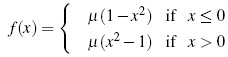
and we take µ < 0 to be the bifurcation parameter.

We start by recalling that x is a virtual fixed point of f if f (x)= x and x does not belong to the domain of f , as discussed by O. Eriksson et al. [14]. If a point x exists such that f (x)= x, and x belongs to the domain of f then x is said to be a fixed point, and its orbit consists of a single element. On the other hand, if n ∈ N exists such that fⁿ(x)= x and f^k(x) ≠ = x, for each 0 < k < n, then x is a periodic point of f with period n. If x is a periodic point of period n ∈ N then the orbit of x consists of exactly the n elements {x, f (x), f² (x),...f^n-1 (x)}.

In the case where the positive orbit of a point y is infinite, the question arises whether the sequence of iterations of y converges to a periodical point of the function, in addition to the influence of the parameters of the function on such a convergence. As usual, the set of points of the domain of f whose orbit converges to a fixed point x is called the basin of attraction of x and is denoted by Bx. If that set contains only the point x it is said that x is a repeller or unstable fixed point. Otherwise, x is called an attractor or stable fixed point.

2.1 Fixed Points

For x ≤ 0, f has a fixed point x₂:

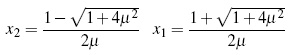
with −1 < x₂ < 0 and 1 < x₁.

For x ≥ 0, f has a fixed point z₁ and a virtual fixed point z₂, where z₁ = −x₁ and z₂ = −x₂, such that:

z1 < &minus 1 and 0 < z2 < 1

By the derivative criterion x1 and z1 are unstable.

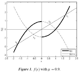
In Figure 1 the fixed points for f (x) may be observed.

3. Results and Discussion

3.1. Orbits of Period Two

To find the basin of periodo two, or 2-cycles, we set f²(x) = x. From the definition of f, it can be seen that

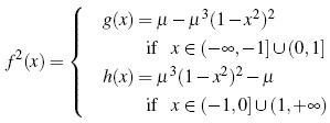
The virtual fixed points of f (x), Λ1 = {x2,z2}, form a 2-cycle as shown in Figure 2. Note that f ²(x2)= h(x2)= x2 and f ²(z2)= g(z2) = z2

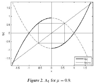
By the derivative criterion we have that if µ, the 2-cycle Λ₁ is unstable, and if 0 , the 2-cycle es stable.

To find the basin of attraction of Λ₁ we require the fact that f² is increasing, as well as the following lemmas.

Lemma 1. If x ∈ (0,z2) then gⁿ (x) ∈ (0,z2) for all n ∈ Nand the sequence (gⁿ(x))_n is increasing in this interval.

As 0 < x < z2, then 0 < g(0)= µ − µ³ < g(x) < g(z2)= z2 and by induction, it follows that 0 < gⁿ(x) < z2. Now, because

then z1 < 0 < x < z2 and (∀ x ∈ R) (−µ³x² + µ²x −µ + µ³ < 0) we have that g(x) − x > 0. Hence, because f² is increasing, g is also increasing; consequently 0 < gⁿ (x) < gⁿ⁺¹(x) < z2

Lemma 2. If x &isin (0, z2) then gⁿ (x) → z2.

By Lemma 1, there is an L > 0 such that lim_n→∞ g_n (x) = L. Suppose that L < z2. Because L g (L) and g(L) < µ. Let

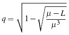
Then q < g(q)= L. For ε = L−q there exists N ∈ N such that ∀ n > N &124;gⁿ (x) − L&124; > ε. Thus, L − gⁿ (x) = &124;gⁿ (x) − L&124; < ε,0 < q < gⁿ (x) < z2 and because g is increasing, then L < gⁿ⁺¹ (x) for x ∈ (0,z2), which is a contradiction. Hence, limⁿ →∞ gⁿ (x) = z2.

Proposition 1. (0,1] ⊆ B_z2

By Lemma 2 we have that (0,z2] ⊆ Bz₂. Inan analogous way, it is shown that, if x ∈ (z2,1] then gⁿ (x) −→ z2.

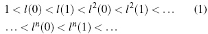
To find the remaining intervals of the basin of attraction of z2, we define the function l with domain R⁺ ∪{0} as l(z)= . We have that l(z)= h⁻¹ (z) for z > 1 and l(z) is increasing in z ∈ (1,x1). So, it can be seen that the function l satisfies the relation 1 < l(0) < l(1). From this inequality, and using the fact that l is increasing, it follows that:

Now, we will prove that lⁿ (1) −→ x1 whenever n → +∞. Because lⁿ (1) is increasing and bounded, there exists an L such that lim_n→∞ l ⁿ(1)= L. Assume that L < x1 and let ε = L − h (L) < 0. There exists an N ∈ Nsuch that ∀ n < N, &124;l ⁿ (1) − L&124; < ε. Hence L − l ⁿ (1) < L − h (L) and applying h we have that 0 < h(L) < l ⁿ(1) < x1. So 0 < L < l ⁿ⁺¹(1) which is a contradiction.

In an analogous way, it may be seen that l ⁿ(0) −→ x1.

From the last two observations, it follows that the length of the intervals (l ⁿ (0),l ⁿ(1)] tends to zero when n → +∞.

Proposition 2. ∪_n∈E (− lⁿ⁺¹ (0), − lⁿ (1)] ⊆ B_z2.

Let x ∪_n∈N(lⁿ (0), l ⁿ (1)] and x ∈ (l^k (0), l^k (1)] for some k ∈ N. Then, l^k−1 (0) < h (x) ≤ l^k−1 (1) and because h is increasing, applying h in the last inequality k − 1 times results in 0 < h^k (x) ≤ 1. By Proposition 1, it follows that h^k (x) ∈ B_z2.

A similar line of reasoning leads to the following result:

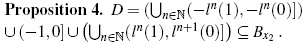
Proposition 3. ∪_n∈N (− lⁿ⁺¹ (0),− lⁿ (1)] ⊆ B_z2.

A similar line of reasoning leads to the following result:

Propositions 3. ∪_n∈N (− lⁿ⁺¹ (0), − lⁿ (1)] ⊆ B_z2.

From propositions 1, 2 and 3 we have that

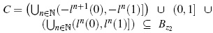
In fact C = B_z2, as we shall see further on.

Using mathematical induction, we see that − fⁿ (x)= fⁿ (−x). Now, let x ∈ Bz_z2 and we shall show that −x ∈ B_x2 for all n ∈ N with x = ≠ lⁿ (1) and x ≠ lⁿ (−1). If x ∈ B_z2 then fⁿ (x) → z2, − fⁿ (x) → −z2 and therefore fⁿ (−x) → x2. If x = 0 then f (0)= µ³ − µ and because −1 < µ³ − µ < 0, we have that 0 ∈ B_x2.

Finally, if x ∈ D then −x ∈ C so −x ∈ Bz₂, leaving us with x ∈ Bx₂.

We shall now look at the basin of attraction of the 2-cycle Λ1.

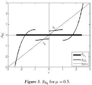
Proposition 5. BΛ₁ = Bx₂ ∪Bz₂ =(z1,x1) with Bx₂ ∩ Bz₂ = Ø.

Because Bx₂ ⊆ (z1,x1) and Bz₂ ⊆ (z1,x1), it follows that Bx₂∪ Bz₂ ⊆ (z1, x1). Now, let x ∈ (z1,x1) and consider the case where x ∈ (0,x1). For ε = x1 − x there exists n1 ∈ N such that, for all n > n1, &124;lⁿ (1) − x1&124; < ε. Hence x < lⁿ(1) and consequently, x ∈ Bx2 ∪ Bz2.

In a similar way, the inclusion for the case x ∈ (z1,0] may be shown.

Figure 3 shows the basin of attraction of Λ1 obtained numerically.

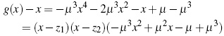
Next, we characterize the remaining 2-cycles of the system. For this purpose, let h (x) = x, initially, that is:

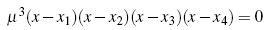
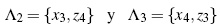
where x3 = and x4 = For g(x) the fixed points are z1, z2, z3 = -x3 and z4 = -x4.

If 0 < µ < , then x3, x4, z3 and z4 are not real. Hence, there are no more 2-cycles.

If µ = , then x3 = x4 = x2 = and z3 = z4 = z2 = , , and we again obtain the 2-cycle Λ1.

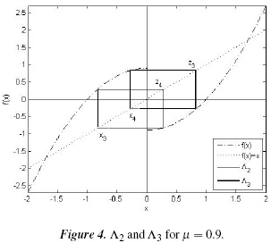
If < µ < 1, we have −1 < x3 < x4 < 0 and 0 < z4 < z3 < 1. So x3 and x4 belong to the domain of h (x) and z3, z4 belong to the domain of g (x).

Consequently, we have the following additional 2-cycles:

By the derivative criterion, both 2-cycles are stable. The 2-cycles Λ2 and Λ3 are shown in Figure 4.

A similar construction for the basin of Λ1 leads to:

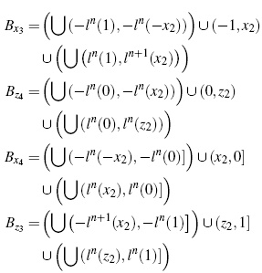
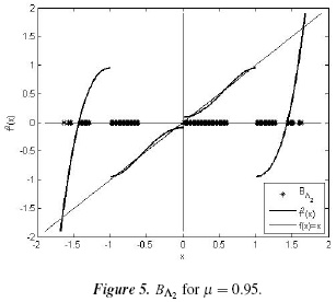
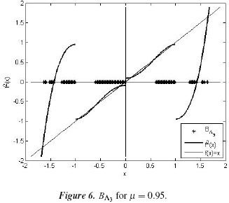
So, BΛ₂ = Bx₃ ∪ Bz₄ and BΛ₃ = Bx₄ ∪ Bz₃, as illustrated in Figures 5 and 6.

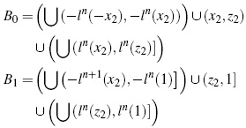
If µ = 1, then x3 = −1, x4 < = z4 and z3 = 1, in which case the fixed point x3 does not belong to the domain of h(x); nevertheless, we have found the stable 2-cycle Λ4 = {0,1} whose basin of attraction is B₀ ∪ B₁, where

If 1 < µ, then x3 < −1, 0 < x4 < 1, 1 < z3 and −1 < z4 < 0. Consequently, these points do not belong to the domains of h(x) and g(x), respectively, so these cases are not considered.

Finally, if x < x1 it may be seen that fⁿ (x) → +∞; additionally, if x < z1 then fⁿ (x) →−∞. Hence, if x ∈ (− ∞, z1) ∪(x1, + ∞) it follows that x does not belong to the basin of attraction of any 2-cycle.

3.2. Numerical Calculations

To obtain the basins of attraction of Figures 3, 5 and 6 numerically, the following procedure was used: a point x0 in the domain of f ² was taken, and its positive orbit {x0, f(x0),...,fⁿ(x0)} was found, with n = 1000. If the difference between fⁿ (x0) and a fixed point x of f ² was less than ε = 10⁻³ then x0 was taken as a point in the basin of attraction of x.

3.3. Bifurcation Diagram

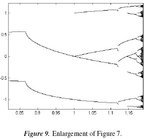
It is well-known that the dynamics of a system may change drastically when one or more of its parameters vary. This qualitative or structural change is known as a bifurcation. In general, bifurcation theory studies the structural changes undergone by dynamical systems when their parameters change, as discussed elsewhere [15]-[16]. These types of changes may be appreciated in their respective bifurcation diagrams, as the bifurcation diagram determines whether the system converges to an n-cycle or exhibits random behavior. In Figures 7 and 8, a bifurcation diagram is shown for the system under study, where the horizontal axis represents the values of the parameter µ and the vertical axis represents the iterations of the variable x. An initial condition x0 is chosen, its positive orbit {x0, f (x0),...,fⁿ (x0)} is found with n = 2000 for each value of µ, and the last 100 iterations are plotted, according [17].

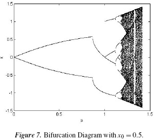
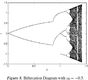
From the diagram, it can be seen that for certain values of the bifurcation parameter, two coexisting stable 2-cycles are present. Then, depending on what basin of attraction the initial condition belongs to, the corresponding 2-cycle will appear in the bifurcation diagram. These diagrams show that, for 0 < µ < ≈ 0:866 there exists a stable 2-cycle Λ1 = {x2, z2} formed by the virtual fixed points of f (x). When µ = , the first bifurcation occurs, and the former 2-cycle becomes unstable and gives rise to two 2-cycles, Λ2 and Λ3, symmetrical with respect to the point x = 0 (as may be seen in Figure 4).

At µ = 1 the second bifurcations appears, called a border-collision bifurcation because when µ → 1, then x4 → 0 and z4 → 0; additionally, at µ = 1, x4 and z4 collide at x = 0 and disappear to give rise to a 4-cycle. This process is repeated for the bifurcation diagram windows where f (x) does not present chaotic behavior. In Figure 9, an enlargement of the diagram is shown where these two bifurcations occur.

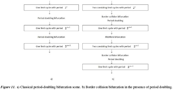
In Figure 11 a comparative analysis is performed between a bifurcation due to period doubling and a bifurcation due to border collision in a scenario with period doubling bifurcation, based on [10].

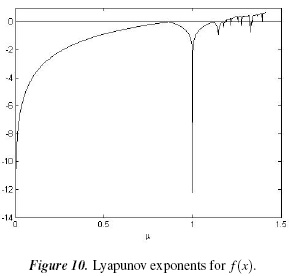
3.4. Lyapunov Exponents

Lyapunov exponents may be used to measure the future separation of two orbits which were initially very close to each other. In general, the analytic calculation of these exponents is extremely involved, requiring the use of numerical calculation. If the orbits were initially very close to each other and remain so in the future, then the associated Lyapunov exponents will all be negative. However, if the paths diverge, there will be at least one positive Lyapunov exponent. In this manner, Lyapunov exponents are related to the system's sensitivity to initial conditions.

Lyapunov exponents can be calculated numerically as in [18], with the following method:

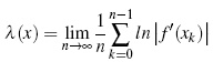
where xk = f ^k(x).

The Lyapunov exponents for f (x) with the initial condition x0 = 0.5 are shown in Figure 10. It can be seen that, for certain values of the parameter µ, there exist positive Lyapunov exponents. Because the system evolves in a bounded fashion in the state space, it can be concluded that the system exhibits chaotic behavior [17, 19].

4. Conclusions

Piecewise smooth one-dimensional applications may generate complex dynamics, such as the coexistence of attractors and border-collision bifurcations, as discussed elsewhere [5, 7].

For the system considered herein, the function f (x) has two unstable fixed points and two virtual fixed points, if 0 < µ ≤ , there is only one stable 2-cycle formed by the virtual fixed points; if < µ < 1, then the existing stable periodic orbit becomes unstable, giving rise to two stable 2-cycles; if µ = 1, the two 2-cycles Λ2 and Λ3 collide and form an orbit with period 4. Finally, if 1 < µ, the 2-cycle vanishes.

The stability analysis of orbits with periods one and two was performed using the derivative criterion, together with the respective basins of attraction of the orbits, showing that the orbits are formed by a countable collection of intervals whose lengths tend to zero.

Simulations were carried out using Matlab to numerically study the dynamics of the system, and the agreement of simulations with analytic results was confirmed.

Acknowledgements

This work was supported by Universidad Nacional de Colombia Sede Manizales, Research Group: Cálculo Científico y Modelamiento Matemático y La Dirección de Investigaciones Sede Manizales (DIMA).

References

[1] S. Wiggins, "Introduction to Applier Non-linear Dynamical Systems and Chaos", Springer-Verlag, Second Edition, 2003.         [ Links ]

[2] M. di Bernardo, M.I. Feigin, S.J. Hogan, M.E. Homer, "Local Analysis of C-Bifurcations in n-Dimensional Piecewise Smooth Dynamical Systems", Chaos, Solitons and Fractals, vol. 10, no. 11, pp. 1881-1908, 1999.         [ Links ]

[3] M. di Bernardo, C.J. Budd, A.R. Champneys, P. Kowalczyk, "Piecewise-smooth Dynamical Systems", Springer Verlag London Limite, 2008.         [ Links ]

[4] M. di Bernardo, A. Nordmark, G. Olivar, "Discontinuity-Induced Bifurcations of Equilibria in Piecewise-Smooth and Impacting Dynamical Systems", Physica D, vol. 237, no. 1, pp. 119-136, 2008.         [ Links ]

[5] B. Robert, C. Robert, "Border Collision Bifurcations in a One-Dimensional Piecewise Smooth Map for a PWM Current-Programmed H-Bridge Inverter", International Journal of Control, vol. 75, no. 16 & 17, pp. 1356-1367, 2002.         [ Links ]

[6] Y. Do, S.D. Kim, P.S. Kim, "Stability of Fixed Points Placed on the Border in the Piecewise Linear Systems", Chaos, Solitons and Fractals, vol. 38, pp. 391-399, 2008.         [ Links ]

[7] P. Jain, S. Banerjee, "Border-Collision Bifurcations in One-Dimensional Discontinuous Map", International Journal of Bifurcation and Chaos, vol. 13, no. 11, pp. 3341-3351, 2003.         [ Links ]

[8] W. Zheng, "Chaoization and Stabilization of Electric Motor Drives and Their Industrial Applications", Tesis Doctoral, The University of Hong Kong, 2008.         [ Links ]

[9] G. Yuan, S. Banerjee, E. Ott, J.A. Yorke, "Border-Collision Bifurcations in the Buck Converter", IEEE Transactions on Circuits and Systems-I: Fundamental Theory and Applications, vol. 45, no. 7, pp. 707-716, 1998.         [ Links ]

[10] V. Avrutin, M. Schanz, "Border-Collision Period-Doubling Scenario", Physical Review E, vol. 70, no. 2, 2004.         [ Links ]

[11] M.A. Hassouneh, E.H. Abed, S. Banerjee, Feedback Control of Border Collision Bifurcations in Two-Dimensional Discrete-Time Systems, Reporte Técnico, University of Maryland, 2002. Disponible en: http://hdl.handle.net/1903/6273.         [ Links ]

[12] S. Brianzoni, R. Coppier, E. Michetti, "Complex Dynamics in a Growth Model with Corruption in Public Procurement", Discrete Dynamics in Nature and Society, vol. 2011, 2011. doi: 10.1155/2011/862396.         [ Links ]

[13] B. Routroy, P.S. Dutta, S. Banerjee, Border Collision Bifurcations in n-Dimensional Piecewise Linear Discontinuous Maps, Cornell University Library, 2006. Disponible en: http://arxiv.org/abs/nlin/0601038.         [ Links ]

[14] O. Eriksson, B Brinne, Y. Zhou, J. Bjorkegren, J. Tegnér, Deconstructing the core dynamics from a complex time-lagged regulatory biological circuit The Institution of Engineering and Technology, 2009, doi: 10.1049/iet-syb.2007.0028.         [ Links ]

[15] Robert L. Devaney, An introduction to Chaotic Dynamical Systems, Second Edition, Addisson Wesley Publishing Company, Inc. 1989.         [ Links ]

[16] Y.A. Kuznetsov, Elements of applied bifurcation theory, Springer Verlag, New York, 2004.         [ Links ]

[17] D. Gulick, Encounters with Chaos, McGraw-Hill, Inc. 1992.         [ Links ]

[18] B. Brogliato, Nonsmooth Mechanics., Springer Verlag, 1999.         [ Links ]

[19] S. Banerjee, G.C. Verghese, Nonlinear phenomena in power electronics, Eds. IEEE Press, Piscataway, 2001.         [ Links ]