1 Introduction

As the time goes by, identification of circuit and excitation parameters of synchronous generators has been approached from several perspectives that involve parametric estimation techniques and states, in order to find time constants, gains and limits which the generator operates either connected to the electrical network or off-line. These techniques could be classified into the categories of estimation by least squares and Kalman Filter. The modeling of both circuit parameters and excitation systems present in synchronous machines has a fundamental role in the stability of the power systems present in the national interconnected system. The reference ¹ proposed practices with models of suitable excitation systems in stability studies for large-scale power systems such as the synchronous generator, while the generation of circuit parameters of the generator is contemplated in ². Owing to the idea of this research work is focused on estimating the parameters of a synchronous generator at laboratory scale, so it is taken as reference, ².

In order to carry out the comparative study between the two techniques of identification machine parameters, it must be taken into account that the problem has been approached according to its different variants, on one side the researches carried out in ^{3 4 5 6 7 8 9}, focus their job on estimate circuit parameters of the synchronous generator which have been object of abundant study. Whereas in ^{10 11 12 13 14 15 16}, have been estimated excitation parameters by different techniques, and similarly there are variety of publications recorded. On the other hand, to obtain the estimation of either the circuit or excitation parameters of the synchronous generator, it is based on obtaining a model that depends on the nature of the machine used. This model can be linear as shown in ^{4 5 11 10 17 14 9}, or no linear as used in ^{18 6 12 7 13 8 19 16 20}. Also, the various investigations in their phase of data collection used different types of measurements to carry out the parameters identification, these measurements were made using data time ^{18 3 4 5 6 10 7 8 17 14 21}, frequency data ^{19 15 9}, or with phasor measurement units (PMU) ^{11 12 13 16 20}.

Identification techniques are essentially based on recursive and non-recursive estimation, they are distinguished because in first one the current estimation of the parameters is made based on a previous estimate. Whereas in certain practices it is opted to make a joint estimation between parameters and dynamic states of the system, as it usually happens in the studies where the technique used is the Kalman filter or any of its variations. In ^{18 5 10} recursive least squares was chosen as the method for estimating the synchronous generator parameters and ¹⁴ used nonlinear least squares, these methods generate few computational costs but yield high prediction if the noise affects the measurement. Other particular methods as Levenberg-Marquadrdt ¹⁹, output error method (OEM) ⁴ and error prediction ¹⁵ were carried out to estimate the machine parameters, or the case in ⁹ where the frequency and time response methods ⁸ were applied independently. In addition, some authors of recent studies carry out joint estimation of parameters and states using the unscented Kalman filter (UKF) technique ^16,13, extended Kalman fileter (EKF) ¹², or Kalman square root ⁷, these techniques start from a non-linear model and can estimate at most 5 parameters of the synchronous generator, while in ²⁰ the unknown input Kalman filter (UIKF) only made the estimation of four dynamic states of the machine. Over the years, many research studies have resulted in synchronous generator models closer to the real model, however a detailed comparison between parameter estimation techniques has not been carried out to establish which of these offers the best results to obtain models and parameters in relation to the other techniques.

The article is structured as follows: section 2 describes the mathematical model of the generator, section 3 is dedicated to the recursive least squares and section 4 presents the Kalman filter algorithm, followed by the results presented in the section 5 and ending with the conclusion of the article in the section 6.

2 Synchronous generator model

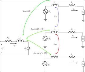
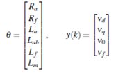
First, it is presented the equivalent circuit of a synchronous generator in abc coordinates, where Va,b,c, ia,b,c and Ya,b,c are respectively the winding voltage, current and linkage flux on armature, Vf, if Yf are the same but in the field. While L _a is the armature-phase inductance, L _ab is the armature phase-phase mutual inductance, L _m is the peak armature-phase to field-winding mutual inductance, Lf is the field-winding inductance, R _a is the armature phase resistance, Rf is the field-winding resistance and 6 is the electrical angle between the magnetic axis of phase a and the magnetic axis of the field winding. Applying the voltage Kirchoff law to each electric circuit on Figure 1.

Figure 1 Equivalent circuit in abc coordinates. 

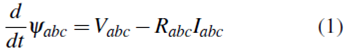
where flux and current vectors can be associated as:

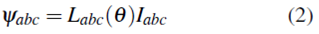
In the previous equations, the inductance matrix Labc is time dependent, so it is necessary to apply Park transformation multiplying both sides of the equation (2) by a term that disappears the dependence. Thus the L _abc turns to L_dq0 and this is the new equation with a state space representation:

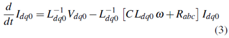
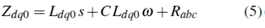
where m is rotor electrical angular velocity and C is a zeros matrix with C_1;2 - 1 and C_2;1 - -1, with a constant value of m, the equation 3 could be written as voltage matrix applying Fourier transformation:

So the previous equation can be written as a impedance matrix

3 Recursive least squares algorithm

Basic RLS algorithm seeks to minimize the squares of the prediction errors sum, by the following discrete representation of a dynamic system

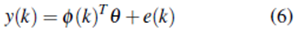
according to equation (4) it defines the outputs and parameters vectors as:

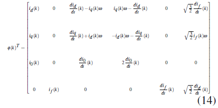
and the regression matrix set as, see equation 14. Note that it was not necessary to use the discrete steps but in exchange derivatives of current signals in relation with the time must be calculated whereby the least squares method is used. These are the steps for designing a recursive least squares algorithm.

• Prediction error

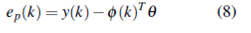
• Gains vector

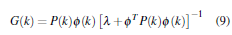
where P is the covariance matrix that must be initialized when k - 0, thus:

meanwhile the forgetting factor is considered with a value close to one (X = 0.999), which generates a slow convergence to the value of the parameters but greater immunity to noise.

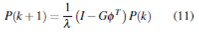
Covariance matrix in the step k+ 1

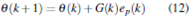
Update parameters

4 Kalman filter algorithm

For this particular case was considered the following state space representation of a discrete system:

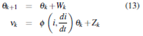
where W is the random process noise and Z is the measurement noise. Kalman filter can accommodate parameters estimation by using the following equations

Prediction stage. Projection of the state:

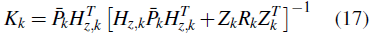
Projection of the covariance error:

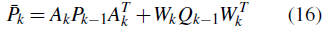
State correction. Kalman Gain

State correction:

Covariance error update

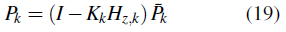
Where:

The value of process noise variance Qk was set in zero, since there is a certain reliability that the parameters at the step k + 1 are equal at the step k due to the proposed model. Whereas the measurement noise variance is a identity matrix. Previous equations were implemented in MATLAB.

5 Results

Note that both methods require regression matrix 14 so they are very similar and only differ in their equations. Two experiments with simulated and real data were considered, for the first one it was designed a virtual generator model and one vector with random values of the parameters. In the other hand instead, current and voltage signals are measured from a laboratory machine with a acquisition data software.

5.1 Simulated data

The initial value of the parameters was set as zero and different values of white noise variance were added to the three-phase voltage and current signals in order to check the quality of the algorithms. Then the time convergence of the estimated parameters is shown.

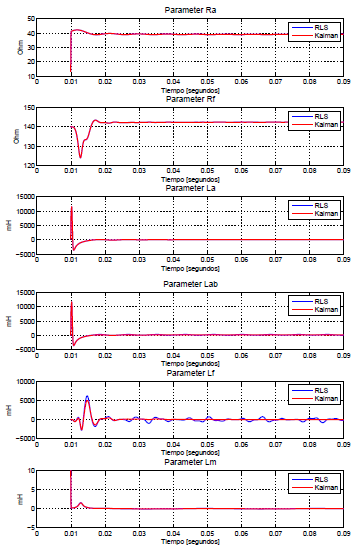
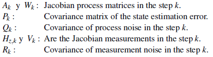
Figure 2 shows great similarity between RLS and Kalman filter because of both estimate a closer value of real parameters, however recursive least squares (blue line) always present a more oscillatory time response than Kalman especially in the inductive parameters. Furthermore the estimated parameters with both algorithms are shown in the following Table 1.

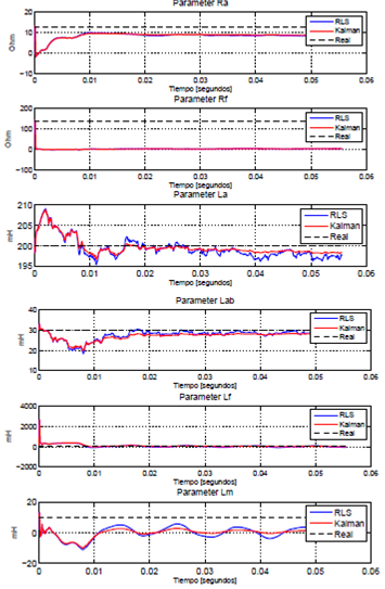
Figure 2 Convergence of the estimated parameters by the algorithms with 1 as the value of white noise variance. 

Table 1 Estimated parameters with both methods with different values of white noise variance 

Parameter	Ra	Rf	La	Lab	Lf	Lm
Virtual	13	140	200	30	80	10
White noise variance= 0,01
RLS	12.91	93.01	200.10	30.03	22.37	7.04
Kalman	12.96	94.53	199.72	29.71	67.43	6.95
White noise variance= 0,1
RLS	12.34	24.34	200.65	30.39	-54.44	1.22
Kalman	12.37	22.46	199.22	29.19	30.39	1.61
White noise variance= 1
RLS	8.21	4.28	197.54	28.62	-60.72	-0.04
Kalman	8.73	3.43	198.35	28.06	15.32	0.49
White noise variance= 2
RLS	6.04	1.48	201.57	29.79	-71.58	-0.33
Kalman	6.27	1.23	202.99	30.12	16.52	0.66
White noise variance= 5
RLS	3.39	0.73	200.77	28.06	-55.37	0.07
Kalman	3.52	0.88	200.95	27.37	16.37	0.17

Resistance parameters unities are Ohms and inductive unities are mils-Henri. Note that Kalman filter has greater noise immunity due to considers this component in his equations and always recover a closer parameter value to real, on the contrary recursive least squares quality decreases as white noise variance increases. Hence Kalman filter would be the best option.

5.2 Real data

A data acquisition of voltages, currents and rotor velocity with Arduino DUE was carried out in three different scenarios, 1000 samples was acquired and the sampling time was 100 micro-seconds. After processing the obtained signals the methods were compared. The machine must be connected as a engine because of the impedance equation 5 and all the the system will see as a load.

5.2.1 First scenario: Different values of Vf

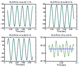
A manual variation of the excitation machine voltage was made and the following fit between real and predicted signal was obtained. The example shows the results for Vf - 20 volts.

Figure 3 shows the performance of the algorithms to predict the three-phase signals, while the percentage of zero in the field voltage is due to the resolution of the sensor used in that channel since it fails to sense an AC induced voltage value in such a large DC component. Then it is presented the estimated parameters time convergence.

Figure 3 Fit between measured signal (blue) and predicted signal (green). 

Here, the great similarly between the estimation methods because of the identified parameter value and their time signal evolution. Thus it is necessary to see the estimated parameters on different values of the field voltage. In the Table2 it can appreciate how the quality of the identification with both methods decreases as the field voltage increases, that may due to the magnetic saturation in the iron structure of the machine, in low excitation voltages the algorithms be able to recover similar values of the machine parameters.

Table 2 Comparison between the algorithms with different values of Vf 

Recursive Least Squares
Vf ( v) Parameter	5	10	20	30	60	120
R a ( Ohms)	40.25	39.07	35.77	38.68	23.87	14.67
R f ( Ohms)	142.63	141.86	142.52	114.53	140.09	143.54
La ( mH)	284.42	-31.32	7.59	44.08	-295.88	-92.03
L ab (mH)	490.38	171.69	206.12	258.69	-146.83	37.87
Lf ( mH)	-63.25	487.83	43.51	-33.79	-441.24	-1964.04
L m (mH)	0.03	-0.06	0.02	0.13	-0.16	0.38
Kalman filter
V f ( v) Param	5	10	20	30	60	120
Ra ( Ohms)	40.87	39.02	35.79	38.69	23.64	14.89
Rf ( Ohms)	142.60	142.44	142.56	114.53	139.70	141.70
La ( mH)	191.70	33.49	45.63	121.74	-258.55	-167.92
L ab (mH)	403.52	235.55	243.28	335.42	-109.84	-37.75
L f ( mH)	7.68	37.86	8.47	-22.24	10.74	-87.34
L m (mH)	-0.01	0.01	0.01	0.03	-0.04	0.07

5.2.2 Second scenario: Line frequency = 50 Hertz

A variable frequency driver was connected in open loop with the machine in order to slow the line frequency down. It is worth to clarify that the delivered voltage signal by the driver is not sinusoidal hence the fit between signals is 0%. The estimated machine parameters are shown in the Table3. Note that despite the aforementioned, the algorithms are able to estimate the value of some parameters since the magnitude of the three-phase voltage is maintained and the only variable that changes its value is the frequency.

Table 3 Comparison between the estimated parameters, the machine operates with 50 ⁽Hz⁾ 

Parameter	RLS	Kalman
Ra ( Ohms)	16.99	13.39
Rf ( Ohms)	141.88	141.79
La ( mH)	-1018.41	204.15
L ab (mH)	-936.69	294.46
Lf ( mH)	-213.49	-149.67
L m (mH)	0.03	-0.05

5.2.3 Third scenario: The machine carries a load

An electro-dynamo is drawn by the motor through a belt. In the same way the acquisition data was carried out and sinusoidal signals of voltage and currents in three phase were obtained. Identified parameters are shown in the following Table 4.

Table 4 Comparison between the estimated parameters, the machine carries a load 

Parameter	RLS	Kalman
Ra ( Ohms)	-11.77	-11.81
Rf ( Ohms)	140.10	140.10
La ( mH)	-112.32	-113.71
L ab (mH)	28.67	27.81
Lf ( mH)	13.62	0.31
L m (mH)	0.02	0.00

Definitely this scenario is not the appropriate to estimate the machine parameters due to the three-phase currents get a very large value and the rotor velocity slows down very much.

6 Conclusion

An alternative methodology was presented to model the synchronous generator to avoid discretization. Both designed algorithms in this work were very similar to estimate the synchronous machine parameters with low excitation voltages getting a great accuracy to the identified values. Kalman filter was slightly higher than RLS because of it considers noise model in the equations, hence the first one presented smaller oscillations in the convergence time figure of some estimated inductances.

Figure 4 Time convergence of the estimated parameters, the machine operates with V _f - 20 volts.