Espanhol (pdf)
 Artigo em XML
 Referências do artigo
 Enviar este artigo por email
 Citado por SciELO
  Citado por Google
  Similares em
SciELO
Similares em
SciELO  Similares em Google
 Permalink
1. Introducción
Continuous on-line measurements such as UV-Vis spectrometry is increasingly applied technique for water quality measurement in sewer systems [1] - [5]. These continuous time series [6]-[8] help to estimate pollutant concentrations in sewer systems and offer real-time control applicability [9]-[13]. Absorbance (essentially surrogate measurements for TSS - Total Suspended Solids or COD - Chemical Oxygen Demand) time series can be used to estimate the dry weather contribution to total TSS and COD loads measured during storm events [15], [15]. In fact, most models of storm weather pollutant loads in combined sewer systems are based on the assumption that total storm event load is the sum of dry and wet weather contributions, with the latter including surface runoff plus possible erosion of deposits accumulated in sewers [16]-[19]. Therefore, during rain events, it is important to distinguish the fraction of flow rate corresponding to dry weather and that corresponding to wet weather. This process, however, is hindered by the fact that the time series may present outliers. Johnson and Wichern [20] define an outlier as "an observation in a data set which appears to be inconsistent with the remainder of that set of data" [21]-[23], [25], [28]. Researches had been used different methodologies to detect the isolated and extremely peak values as PCA by [23], also using statistical procedures based on prior knowledge of the system that produces the data [21], [24]-[28]. Others researches have been applied artificial intelligence and machine learning methodologies [22], [29]-[31]. In addition, lost values, due to obstructions on the sensors themselves or the occasional sensors removal required for maintenance, would be also present; researches have been using different methodologies for infilling missing values in data sets as Artificial Neural Networks (ANN) by [32], Evolutionary Algorithms by [33], Genetics Algorithms by [34], clustering by [35], using PCA by [36], Bayes' theorem [37], linear and non-linear regressions [38]-[40]. Several detection outlier techniques require to obtain a fitted model [41] to assess which are the extremely peaks to be removed and the infilling methods require multivariate information to obtain a model to fill the gaps in data sets.
The methodology laid out in this article detects and removes outliers and fill gaps making the missing values imputation in time series. In theory, the proposed procedure combines statistical values, outlier detection [42], [43], DFT and IFFT to complete time series. Thus, it is used the combination of the Winsorising and DFT procedures to perform the task of detection, removal of outliers and imputing of missing values to maintain the observed periodic behaviour of these time series. In practice, this methodology was applied to three time series at the same number of study sites in Colombia for UV-Vis spectra. Locations of the study sites are as follows: (i) Bogota D.C. Salitre-WWTP (Waste Water Treatment Plant), influent; (ii) Bogotá D.C. Gibraltar Pumping Station (GPS); and, (iii) Itaguí, San Fernando-WWTP, influent (Medellín metropolitan area).
2. Materials and Methods
The spectro::lyserTM UV-Vis sensors deployed at the three Colombian sites are submersible probes with a length of approximately 65 cm and a diameter of approximately 44 mm. Functionally speaking, they register light attenuation (absorbance) on-line in relative continuous time (one signal per minute). These sensors work with a light source provided by a Xenon lamp for wavelengths ranging from 200 nm to 750 nm, with intervals of 2.5 nm [1], [44].
With regard to the duration of the study, i.e. data gathered, the three time series are displayed in Figure 1: (i) Bogotá D.C. Salitre-WWTP, influent (5705 records, one per minute, from June 29th, 2011 at 9:03 h to July 3rd, 2011 at 17:33 h); (ii) Bogotá D.C. Gibraltar Pumping Station (GPS) (35684 records, one per minute, from October 18th, 2011 at 16:17 h to November 11th, 2011 at 11:20 h); and (iii) Itaguí, San Fernando-WWTP, influent (Medellín) (107204 records, one every two minutes, from September 24th, 2011 at 11:08 h to February 20th, 2011 at 10:18 h.
As Figure 1 aptly demonstrates, outliers accompanied our data collection. Outliers, those data that deviate significantly from the majority of observations, may be caused by different mechanisms in relation to normal data [21], [24]-[28]. These different mechanisms include, but are not limited to, factors such as sensor noise, process disturbance and instrument degradation. Relying on a time series tainted by outliers proves to be a source of frustration, as it often leads to misinterpretation and model misspecification. To help offset this aspect of data collection, data pre-processing is a necessary pre-requisite to monitoring data processing [45]. In order to detect and imputing these pesky outliers, the Winsorising procedure, which consists of transforming the original data by limiting extreme values, reduces the effect of possibly spurious outliers [46]. Moreover, Winsorising is known for promoting a smoother filter, allowing researchers to place more weight on the central value of each time window by using a mobile window of values (N) [47], [48]. Such values depend on r, the number of values to be modified, where 2r + 1' equals window size (N); yet, here it is incumbent upon researchers to set the range m of values to be analysed, for m is required to establish the minimum and maximum values for the window range and allow the removal of values beyond the upper or lower limits with regard to m in order to obtain the winsorised data [47]. The process carried out in this investigation can be explained in terms of two multi-part steps.
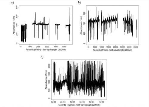
Figure 1 Original time series with outliers and missing values for Salitre-WWTP (a), GPS (b) and San Fernando-WWTP (c) (self- authorship)
The first consists of sorting the data in the selected window from lowest to highest; several visual reviews were done to test values of r and m parameters. These values were defined once was observed the removal of outliers and before the shape of the signal has lost. Then, values below the minimum acceptable value (M inAV ) are removed. M inAV is understood as the value of (m+1)th place for all values in the window. M inAV is represented by Equation 1.
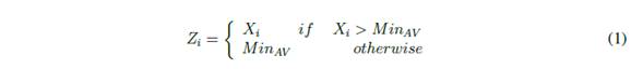
where Xi is the ith window value, MinAV the minimum acceptable value and Zi the resulting values after the removal of values below MinAV . As a result, any value lower (outlier) than Min AV will be replaced. A similar procedure is followed to remove outliers above a threshold MaxAV , which is equal to the value of the (N - m)th place of all values in the Zi window see Equation 2.

where Zi is the ith window value, MaxAV the maximum acceptable value and Yi the resulting values after removal. It is worth mentioning here that the above, Equation 1 and Equation 2, adapts the method proposed by [46].
Once the corrected time series (without outliers) is obtained, a DFT procedure to complete the time series can be applied. With DFT, the time series is calculated to facilitate the switch from the time domain to the frequency domain. This technique involves the conversion of a finite number of equally spaced samples (discrete points) into a number of coefficients that stem from a finite combination of complex sinusoid components. Doing so ensures that the frequency domain is comprised of the same number of sample values as the previous time domain [48], [49].
Equation 3 details this conversion. DFT likewise ranks components based on their importance, with importance determined by component amplitude. After ranking, components are eliminated from lower to higher importance, leaving only the most significant harmonics (10%) in the resulting values. Finally, the Inverse Fast Fourier Transform (IFFT) is utilized to convert complex sinusoids (harmonics) into a finite number of discrete points. This movement represents a return to the time domain (as opposed to the time to frequency shift found in the initial DFT process), as shown in Equation 4. For more details, see [50].


where n is the current sample that is analysed, N is the total number of time samples taken, k is current harmonic (frequency) that is considered (0 Hertz up to N - 1 Hertz), xn is the value of the time series at time n and Xk is the amount of frequency k in the signal (complex number) [49].
The Winsorising process (first step) is applied to the absorbance time series. However, outlier values may still remain; these values must be dealt with. Having outlined the first step, we can proceed to the second step. The procedure obtains the median value from the entire dataset; next, any upper and lower values within median value +/- one standard deviation range will be discarded (referred to round one). In fact, one standard deviation is used because the time series is highly affected by outlier values that remain after the first round and before DFT is applied. Consequently, the dataset must be switched from the time to the frequency domain. This switch, done with values present in the data set prior to the first missing values gap, naturally leads to the selection of the two most important harmonics. These two harmonics are selected "naturally" insofar as they reproduce the pattern and dynamic of the events. In effect, it is possible to reproduce the outliers if more than two harmonics are included. By virtue of IFFT, the data is translated from the frequency domain back into the time domain. Afterwards, the resulting time series is used to complete the first gap of missing values. Then, the median value from the entire dataset is again obtained and any upper and lower value within median value +/- two standard deviations range will be taken out (referred to as round two).
On account of Winsorising, along with the two rounds of standard deviation refinement, the effect of outliers at this stage has been attenuated but not fully counteracted. So, the DFT process is run again with only the two most important harmonics applied, followed by another run of IFFT. The resultant time domain values are then able to facilitate the completion of the first missing values gap. When this process is completed, the first gap (missing values) will have been complemented. Therefore, the process described up to this point is brought to bear on the corrected data ranging from the starting point (including the first "completed" gap) to the beginning of the second gap. The same is done with all the corrected data from the initial point to the start of the third gap (including the "completed" first and second gaps) and so on.
Finally, DFT is applied to the resulting time series and the 10 % of the most important harmonics are used. Going from the frequency domain back to the time domain is once again done with the IFFT process. At this stage, new values imputing either outliers or missing values have the same, or almost the same, shape as the original time series, granting the "macro" vision of the time series coherence. To follow the intricacies of this process, readers can consult the flow diagram shown in Figure 2.
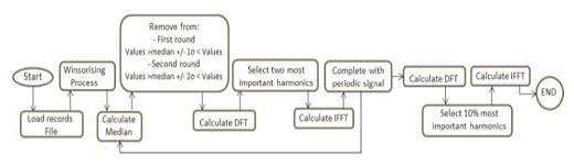
Figure 2 Flow diagram depicting detection and removal of outliers and replacement of missing values (self-authorship)
However, as would be expected, the proposed procedure was tested to determine its validity. To this end, continuous subsets of absorbance time series with no outliers and no missing values were intentionally removed from the original time series. In order to assess the accuracy of the method proposed, the mean absolute percentage of error (MAPE) was used as shown in Equation 5, where Val real is the original time series value and Val rep is the replaced time series value.

3. Results and Discussion
For all the study sites, the Winsorising process, coded with R statistical language [51], was applied using a value of ten (10) for r and m parameters to build the window size and find the minimum and maximum acceptable values. Several value combinations of r and m parameters were verified, and the best results using r and m proved to be a value of ten (10). Although using a bigger window size with 20, 30, 50 or 100 as values for the m parameter, in addition to a lower r value compared with m, effectively eliminates outliers, but the shape of the resulting time series is reminiscent of stair steps (thereby losing its resemblance to the original shape of the time series-Figure 3.
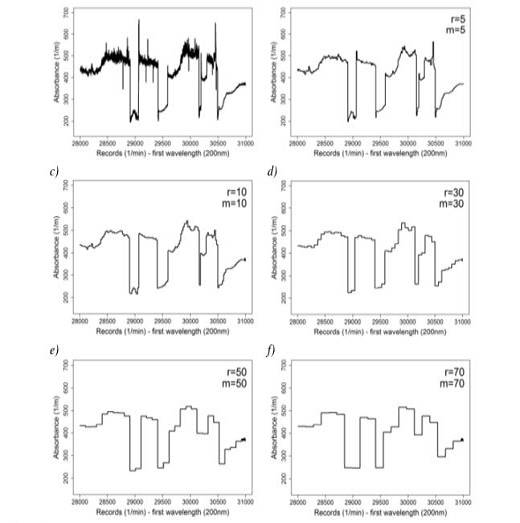
Figure 3 Comparison of different r and m Winsorising parameter values for the GPS Absorbance time series (section spanning values 28000 to 31000) with original (a), r = m = 5 selected value (b), r = m = 10 selected value (c), r = m = 30 selected value (d) and r = m = 50 selected value (e), r = m = 70 selected value (f) (self-authorship)
Figure 3 shows a select section of the GPS absorbance time series, which includes values from 28000 to 31000 for the time series. Five different combinations for r and m parameter values were used, which led to the observation of a time series that mirrors the original time series analysed.
Figure 3 demonstrates that although large window size values (30, 50 or 70) for r and m parameters translate into less outlier values, the time series' shape becomes stair-like, losing its similarity to the shape of the original times series (Figure 3, graph a). Thus, using these large window size values would be disadvantageous because an analysis of the last part of the time series (roughly values 30950 until 31000) becomes largely impossible, as observed in Figure 3 (graphs d, e and f).
However, Figure 3 (graph b) shows the results with some outliers. Therefore, 10 was selected as the optimal value for r and m parameters to strike a balance between the analysed window size and the number of outlier values requiring removal. However, given the fact that some outlier values still remain after applying the Winsorising process, the process of applying one and two standard deviations and DFT is repeated to expunge these outliers from the dataset.
As a result, after the final parameter values are selected for window size using the Winsorising process, the last part of the processes indicated in the flow diagram are undertaken Figure 2. The time series for all three study sites after applying this complete process can be seen in Figure 4.
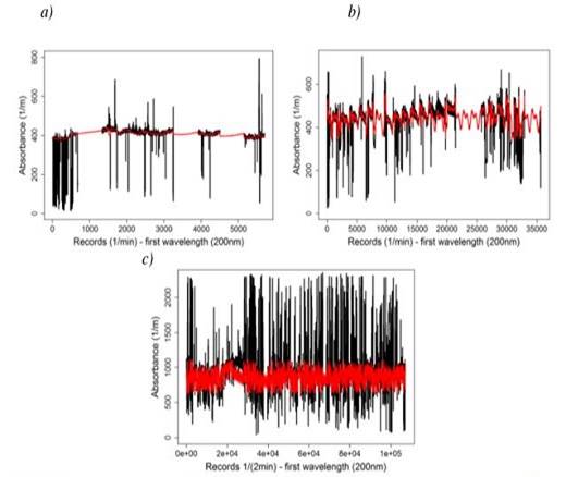
Figure 4 Resulting time series for all three study sites after applying the proposed procedure to Salitre-WWTP (a), GPS (b) and San Fernando- WWTP (c) (self-authorship)
Figure 4's black curve represents the original times series (absorbance) and its red curve the resulting time series. The results obtained are as follows:
Salitre-WWTP: three large gaps of missing values. Although DFT could not be used for imputing missing values in the first gap, it was successfully used for the other two large gaps. Instead of DFT for the first gap, a linear interpolation was used.
GPS: three large gaps of missing values imputed with DFT.
San Fernando-WWTP: longest absorbance time series and greatest presence of outliers (of the three study sites). The entire filter procedure (Winsorising, one and two standard deviations, DFT, IFFT) detected and removed outliers, with DFT reapplied for imputing missing values (see Figure 4, graph c).
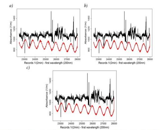
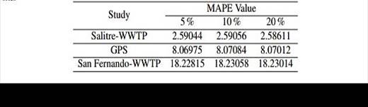
To assess the validity of the results presented by the proposed methodology, continuous subsets (a section) of the absorbance time series without outlier or missing values were removed from the original time series. Similarly, the MAPE (see Equation 5) was used, as shown in Figure 5. Thus, DFT is applied to the resulting time series and according to preliminary test varying from 5 % to 20 % of the most important harmonics (see the appendix). Therefore, it was decided to use the 10 % of the most important harmonics as a sufficient number of harmonics in order to capture de variability of the time series.
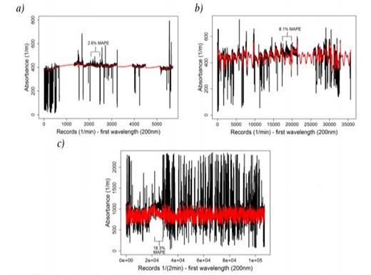
Figure 5 Resulting time series and MAPE values for all three study sites after removal a selecting range values and applying the proposed procedure to Salitre-WWTP (a), GPS (b) and San Fernando-WWTP (c) (self-authorship)
Figure 5 shows the time series (black curve) and the modified-filtered time series (red curve) for all three study sites. Below are the results.
Salitre-WWTP: values 2100 to 2449 were removed, which gives a 2,6 % MAPE.
GPS: values 17500 to 19499 were removed, which gives an 8,1 % MAPE.
San Fernando-WWTP: values 22500 to 27999 were removed, which gives an 18,3 % MAPE.
As the above paragraphs a-c witness, different combinations of values were intentionally eliminated from the original time series (absorbance) at each of the three study sites, in the line with the aforementioned criteria for value exclusion. Overall, a 12 % average of MAPE was obtained.
4. Conclusions
The main contribution of this work is the proposal of a new methodology in order to complete time series with missing values and different characteristics (absorbance), and consists of Winsorising as a step in outlier removal. Also, the application of the DFT and the IFFT, using the 10 % most important harmonics of useful values, which is crucial for its later use in different applications, specifically for time series of water quality and quantity in urban sewer systems. The imputing of missing values process (DFT and IFFT) can be applied to any missing value gap with different length. It was applied the combination of the Winsorising and DFT procedures to perform the task of detection, removal of outliers and imputing of missing values to maintain the observed periodic behaviour of these time series.
The process laid out in this paper consists of Winsorising as a first step in outlier removal. One and two standard deviations were then removed (with the concomitant applications of DFT and IFFT) before repeating DFT and IFFT. As a whole, this process effectively removes all outliers and fills the gaps in the time series.
Likewise, the proposed process relies on small r and m parameter values (where r = m) for window sizes. The three different time series (absorbance) to which the process was applied each exhibited different behaviours and had different sizes. Nevertheless, good results were obtained in terms of what researchers would expect the time series to look like even though there is no dataset with which to compare the time series. Additionally, these results bode well for future applicability in that they offer themselves for application in correcting other hydrologic time series.
DFT allows for the completion of the time series based on the fact that it includes various gap sizes, removes outliers and imputing of missing values. DFT meant lower error percentages at all three study sites, with an error average of 12 %. This reflects what would have likely been the shape or pattern of the time series behaviour had there not been outliers or missing values in the first place.
This work is the starting point to continue with the spectral density estimation process by means of modified rectangular window averaging periodograms with a 50 % overlapping to estimate the periodic behaviour that could be hidden. Also, apply the proposed methodology to different time series with different behaviour and different length as rainfall information, pH, conductivity, temperature, etc. On the other hand, it is necessary to compare the performance of the DFT with other techniques, as machine learning technics (ANN, SVM, AG, etc.) to detect, remove outlier values and impute missing values for time series.