


Services on Demand
Journal
Article
 English (pdf)
 Article in xml format
 Article references
 Send this article by e-mail
Indicators
-
 Cited by SciELO
 -
 Access statistics
Related links
-
 Cited by Google
 -
 Similars in
SciELO
Similars in
SciELO -
 Similars in Google
Share

 Permalink
Revista MVZ Córdoba
Print version ISSN 0122-0268
Rev.MVZ Cordoba vol.19 no.2 Córdoba May/Aug. 2014
ORIGINAL
Validation of models with constant bias: an applied approach
Validación de modelos con sesgo constante: un enfoque aplicado
Salvador Medina-Peralta,1 M.Sc, Luis Vargas-Villamil,2* Ph.D, Jorge Navarro A,3 Ph.D, Leonel Avendaño R,4 Ph.D, Luis Colorado M,1 M.Sc, Enrique Arjona-Suarez,5 Ph.D, German Mendoza-Martinez,6 Ph.D.
1Universidad Autónoma de Yucatán, Facultad de Matemáticas, Apartado Postal 172 Cordemex, C.P. 97119, Mérida, Yucatán, México.
2Colegio de Postgraduados, Campus Tabasco, Periférico Carlos A. Molina Km. 3.5, Apartado Postal 24, C.P. 86500, Cárdenas, Tabasco, México.
3Universidad Autónoma de Yucatán, Facultad de Medicina Veterinaria y Zootecnia, Apartado Postal 4-116 Itzimná, C.P. 97100, Mérida, Yucatán, México.
4Universidad Autónoma de Baja California, Instituto de Ciencias Agrícolas, 17 Boulevard Delta s/n, Ejido Nuevo León, C.P. 21705, Baja California, México.
5Colegio de Postgraduados, Programa en Estadística, Km 36.5 Carretera México-Texcoco, C.P. 56230, Montecillo, México.
6Universidad Autónoma Metropolitana, Xochimilco, Departamento de Producción Agrícola y Animal, Medicina Veterinaria y Zootecnia, Edificio 34, 3er piso, Calzada del Hueso 1100 Col Villa Quietud 04960, México D.F., México.
*Correspondence: luis@avanzavet.com
Received: January 2013; Accepted:November 2013.
ABSTRACT
Objective. This paper presents extensions to the statistical validation method based on the procedure of Freese when a model shows constant bias (CB) in its predictions and illustrate the method with data from a new mechanistic model that predict weight gain in cattle. Materials and methods. The extensions were the hypothesis tests and maximum anticipated error for the alternative approach, and the confidence interval for a quantile of the distribution of errors. Results. The model evaluated showed CB, once the CB is removed and with a confidence level of 95%, the magnitude of the error does not exceed 0.575 kg. Therefore, the validated model can be used to predict the daily weight gain of cattle, although it will require an adjustment in its structure based on the presence of CB to increase the accuracy of its forecasts. Conclusions. The confidence interval for the 1-α quantile of the distribution of errors after correcting the constant bias, allows determining the top limit for the magnitude of the error of prediction and use it to evaluate the evolution of the model in the forecasting of the system. The confidence interval approach to validate a model is more informative than the hypothesis tests for the same purpose.
Key words: Statistics, error, confidence interval, models (Source: MeSH).
RESUMEN
Objetivo. Presentar extensiones al método estadístico para validar modelos basado en el procedimiento de Freese cuando el modelo presenta sesgo constante (SC) en sus predicciones e ilustrar el método con datos provenientes de un modelo mecanístico inédito para la predicción de ganancia de peso de bovinos. Materiales y métodos. Las extensiones fueron la prueba de hipótesis y error máximo anticipado para el planteamiento alternativo y el intervalo de confianza para un cuantil de la distribución de los errores. Resultados. El modelo evaluado presentó SC, una vez eliminado y con un nivel de confianza del 95%, la magnitud del error no sobrepasa 0.575 kg. Por lo que el modelo validado puede usarse para predecir la ganancia de peso diaria de bovinos, aunque requerirá un ajuste en su estructura con base a la presencia de SC para incrementar la exactitud en sus pronósticos. Conclusiones. El intervalo de confianza para el cuantil 1-α de la distribución de los errores una vez que se corrige el sesgo constante, permite determinar una cota superior para la magnitud del error de predicción y usarla para evaluar la evolución del modelo en predicción del sistema. El enfoque de intervalos de confianza para validar un modelo es más informativo que las pruebas de hipótesis para el mismo propósito.
Palabras clave: Estadística, error, intervalo de confianza, modelos (Fuente: MeSH).
INTRODUCTION
The validation of a model is defined as the comparison of the forecasts of the model with the values observed in the actual system to determine whether the model is suitable for the established purpose (1, 2). In the mathematical modeling process, the validation stage with observed data different to those used for obtaining the parameters of the model, plays a fundamental role in the models that will be applied and where forecasts will be used instead of the measurements of the actual system, which may be too costly or difficult to obtain. Barrales et al (3) indicate that in modeling of systems, an essential stage, which poses both conceptual and practical difficulties, is the validation of the models.
Different approaches and techniques have been presented in the literature to validate models. For Mayer and Butler (4), validation techniques can be grouped into four main categories: subjective evaluation (involves a number of experts in the field of interest), visual techniques (comparative graphs), measures of deviation (based on the differences between the values observed and simulated) and statistical tests. In turn, Tedeschi (5) conducted a review of various techniques to evaluate mathematical models designed for predictive purposes: linear regression analysis, adjusted errors analysis, concordance correlation coefficient, several evaluation measurements, mean squared prediction error, non-parametric analysis and comparison of the distribution of the data observed and predicted. Medina-Peralta, Vargas-Villamil (6), indicate that some measures of deviation for validating models contradict with the graphical methods when the model is biased in its forecasts; they recommend using a graphical methods and measures of deviation to validate models.
Freese (7) presented a statistical procedure for validating models without bias (SS) and with constant bias (SC) or proportional bias (SP) in forecasts, which essentially involves determining whether the accuracy and precision of a model or estimation technique meets the requirements of the modeler or user of the model. Rennie and Wiant (8), based on the procedure of Freese (7), proposed the use of an maximum anticipated error or critical error to determine if a model is accurate and precise. Reynolds (9) reviewed the assumptions, deduced the procedure of Freese and extended the results to the case of SS models: a) an alternative approach to the Chi-square test for the accuracy test, b) another critical error based on the alternative approach, and c) a confidence interval (CI) for the quantile 1-α of the distribution of errors. Barrales et al (3) extended the procedure of Freese (7) and the modification suggested by Rennie and Wiant (8) in two ways: a) explicit expression of the procedures of the statistical test under the original approach, for models with SC or SP when the maximum permissible error is expressed as a percentage of the actual values, and b) indication of how to obtain the critical error under the original approach when the model presents SC or SP.
This paper presents the extensions to the statistical method to validate the models proposed by Freese (7), Rennie and Wiant (8), Reynolds (9) and Barrales et al (3) when the model shows SC in its predictions. The method is illustrated with data from a new mechanistic model for the prediction of weight gain in cattle.
MATERIALS AND METHODS
Basic concepts. Let's suppose that there are "n" pairs to compare (Yi, Zi) i=1,2,...,n, where for the pair i, Yi is the observed value, Zi the corresponding predicted value and Di=Yi-Zi the difference between them. On Freese's approach (7) for the determination of the accuracy and precision required, the e values (maximum error allowed in deviations |yi-zi|=|di|) and α (1-α represents the level of accuracy required) specified by the modeler or user of the model, must satisfy that D conforms to a normal distribution with mean zero and P(|D|≤e)≥(1-α) for the model to be acceptable and be considered as sufficiently reliable for the prediction of the system. Thus, a model is accurate or unbiased (SS) when it is true that D conforms to a normal distribution with zero mean.
Determination of constant bias. According to the graphical method used by Barrales et al (3) and Medina-Peralta, Vargas-Villamil (6), the presence of SC will be identified in the predictions of the model. The SC is recognized by a value of the average of differences (![]() ) away from zero and for the graph of the dots (zi, di=yi-zi) forming a horizontal band centered on
) away from zero and for the graph of the dots (zi, di=yi-zi) forming a horizontal band centered on ![]() with a systematic distribution to positive or negative (points above and below the line d=
with a systematic distribution to positive or negative (points above and below the line d= ![]() ) (6, 10). A statistical test for determining if the average of the differences is different from zero would contribute to determine the SC more objectively.
) (6, 10). A statistical test for determining if the average of the differences is different from zero would contribute to determine the SC more objectively.
Validation of models with constant bias. When D has a normal distribution with variance ![]() and mean µD [D~N(µD,
and mean µD [D~N(µD,![]() )] and the model is not accurate for having SC, the precision required P(|D|≤e)≥ 1-α translates into
)] and the model is not accurate for having SC, the precision required P(|D|≤e)≥ 1-α translates into ![]()
![]() once the SC is eliminated by correcting
once the SC is eliminated by correcting ![]() (10). The correction makes the model to accurate and only one statistical test would be precision. The next step is to test the hypothesis with the original approach
(10). The correction makes the model to accurate and only one statistical test would be precision. The next step is to test the hypothesis with the original approach![]() (7, 10) or the alternative approach
(7, 10) or the alternative approach ![]() vs (10). Reject H0 o
vs (10). Reject H0 o![]() with a level of significance α’ if:
with a level of significance α’ if:
![]() (1)
(1)
where in general ![]() represents the quantile γ of the chi-square distribution with "k" degrees of freedom, i.e.,
represents the quantile γ of the chi-square distribution with "k" degrees of freedom, i.e., ![]() . Therefore, if H0is not rejected or
. Therefore, if H0is not rejected or ![]() is rejected, then the model is considered acceptable to forecast under the original and alternative approach, respectively.
is rejected, then the model is considered acceptable to forecast under the original and alternative approach, respectively.
Another approach to evaluate precision is through confidence intervals. Thus, when D~N(µD,![]() ) and the model shows SC, the critical errors corresponding to the original and the alternative approach are:
) and the model shows SC, the critical errors corresponding to the original and the alternative approach are:
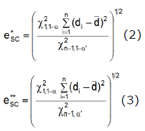
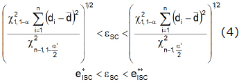
These were obtained by isolating "e" from the rejection regions in equation (1) for H0 and (10); the relationship existing between hypothesis tests and confidence intervals can be found in Casella and Berger (11), which allows constructing one from the other. Therefore, if the modeler or user of the model specifies a value for "e" such that![]() e ≥o e≥ then the model is considered acceptable for predicting the system under the original or the alternative approach, respectively.
e ≥o e≥ then the model is considered acceptable for predicting the system under the original or the alternative approach, respectively.
An estimate with an CI of 100(1-α')% for ![]()
![]() (10), the quantile 1-α of the distribution of errors (e) once the SC is corrected through
(10), the quantile 1-α of the distribution of errors (e) once the SC is corrected through ![]() , is given by:
, is given by:
The CI estimated ![]() means that there is a confidence of 100(1-α')% that the point of the distribution
means that there is a confidence of 100(1-α')% that the point of the distribution ![]() which must be under 100(1-α)% of the absolute errors is located somewhere in such interval. It allows determining with a certain probability an upper bound for the magnitude of the prediction error and use it to evaluate the evolution of the model in the prediction of the system.
which must be under 100(1-α)% of the absolute errors is located somewhere in such interval. It allows determining with a certain probability an upper bound for the magnitude of the prediction error and use it to evaluate the evolution of the model in the prediction of the system.
RESULTS
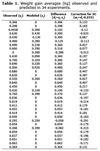
To illustrate the application of the methodology, data from a new dynamic mechanistic model called Wakax POS were used for the prediction of the average weight gain (AWG) per day of bovine animals in a tropical area of Mexico (Table 1). This model was developed by Ph.D. Luis Vargas Villamil of Colegio de Postgraduados, Campus Tabasco, in postdoctoral studies at the Department of Animal Science of the University of California, Davis (UCD). The model Wakax POS describes the biological relationships (digestion, bacterial growth, fermentation and absorption) during the nutrition of cattle fed with sugarcane (CZ) and predicts the average weight gain (AWG) per day in grazing cattle supplemented with CZ, broken corn and/or molasses in a tropical area of Mexico. It consists of 119 states variables that describe the system composed of five sub-models: concentrates, grass, sugarcane, molasses and animal growth. The input variables of the model are: a) live weight; b) consumption of dry matter of corn, molasses, and grass; c) soluble fraction of grass and CZ; d) biodegradable fraction of grass and CZ; and e) ratio of grass and CZ degradation (10).
The goodness of fit tests of Cramer-von Mises (W2=2.172, p<0.003) and Anderson-Darling (A2=10.733, p<0.003) reject (p<0.05) the hypothesis D~N(0,![]() ) with unspecified variance, hence the model is not accurate.
) with unspecified variance, hence the model is not accurate.
The next step is to test D~N(µD,![]() ) with unspecified mean and variance and identify the type of bias. The hypothesis D~N(µD,
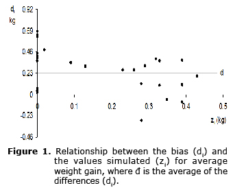
) with unspecified mean and variance and identify the type of bias. The hypothesis D~N(µD,![]() ) is not rejected (p>0.05) (Cramer-von Mises: W2=0.118, p=0.065; Anderson-Darling: A2=0.655, p=0.084; Shapiro-Wilks: W=0.961, p=0.254; Kolmogorov-Smirnov: KS=0.135, p=0.115). In addition, the distribution of the points in figure 1 shows SC, because: (i) the mean of the differences (µD) is different from zero (t=6.092, g.l.=33, p<0.001), and (ii) the points (zi, di) practically form a horizontal band centered on the line =0.233.
) is not rejected (p>0.05) (Cramer-von Mises: W2=0.118, p=0.065; Anderson-Darling: A2=0.655, p=0.084; Shapiro-Wilks: W=0.961, p=0.254; Kolmogorov-Smirnov: KS=0.135, p=0.115). In addition, the distribution of the points in figure 1 shows SC, because: (i) the mean of the differences (µD) is different from zero (t=6.092, g.l.=33, p<0.001), and (ii) the points (zi, di) practically form a horizontal band centered on the line =0.233.
The last step is to apply the correction for SC for the model to be exact and test ~ with unspecified variance.
The goodness of fit tests of Cramer-von Mises (W2=0.122, p>0.25) and Anderson-Darling (A2=0.675, p>0.25) do not reject (p>0.05) the hypothesis ![]()
In this example both approaches were applied, that of the hypothesis tests and that of the confidence intervals, when the model shows SC in its forecasts. Additionally, a 95% CI was calculated for![]() , quantile 1-α of the distribution of errors (e) once the SC is corrected by
, quantile 1-α of the distribution of errors (e) once the SC is corrected by ![]() . With α=α'=0.05 y e=0.5 kg as the maximum error admitted by the modeler or the user of the model, we have that: a)
. With α=α'=0.05 y e=0.5 kg as the maximum error admitted by the modeler or the user of the model, we have that: a) ![]() ≤0.5kg)≥0.95, b)
≤0.5kg)≥0.95, b) ![]() =0.065, c) VSC=25.220 and a level of significance p=0.832 with the original approach (PO) and p=0.168 with the alternative approach (PA). Therefore, the model is considered acceptable for prediction with PO (p>0.05) and unacceptable with the PA (p>0.05).
=0.065, c) VSC=25.220 and a level of significance p=0.832 with the original approach (PO) and p=0.168 with the alternative approach (PA). Therefore, the model is considered acceptable for prediction with PO (p>0.05) and unacceptable with the PA (p>0.05).
The maximum anticipated errors or critical errors are ![]() =0.365 kg and
=0.365 kg and ![]() =0.550 kg; therefore, the modeler or user of the model specifies a precision "e"
=0.550 kg; therefore, the modeler or user of the model specifies a precision "e" ![]() such that
such that ![]() =0.365 kg or
=0.365 kg or ![]() =0.550 kg, then the model will be considered reliable enough in the prediction of the system based on the PO and PA, respectively. Thus, if e=0.5 kg model is considered acceptable for prediction with the PO (e≥0.365 kg) and unacceptable with the PA (e<0.550 kg), which coincides with the statistical decisions obtained with the hypothesis testing approach.
=0.550 kg, then the model will be considered reliable enough in the prediction of the system based on the PO and PA, respectively. Thus, if e=0.5 kg model is considered acceptable for prediction with the PO (e≥0.365 kg) and unacceptable with the PA (e<0.550 kg), which coincides with the statistical decisions obtained with the hypothesis testing approach.
The CI of 1-α'=95% for ![]() is 0.353 kg <
is 0.353 kg <![]() < 0.575 kg, so there is a confidence of 1-α' = 95% that the point of the |W| distribution which is under 1-α = 95% of the absolute errors
< 0.575 kg, so there is a confidence of 1-α' = 95% that the point of the |W| distribution which is under 1-α = 95% of the absolute errors ![]() is located somewhere in the interval (0.353 kg-0.575 kg), i.e., with a probability of 95% the magnitude of the forecast error will not exceed 0.575 kg.
is located somewhere in the interval (0.353 kg-0.575 kg), i.e., with a probability of 95% the magnitude of the forecast error will not exceed 0.575 kg.
With a confidence of 95% of the critical error with the PA and the CI for ![]() , a minimum prediction error of 0.550 kg should be allowed, and it would not exceed 0.575 kg. Hence, the validated model could be used to predict the daily AWG of cattle, although it will require an adjustment based on the presence of SC to increase the accuracy of its forecasts.
, a minimum prediction error of 0.550 kg should be allowed, and it would not exceed 0.575 kg. Hence, the validated model could be used to predict the daily AWG of cattle, although it will require an adjustment based on the presence of SC to increase the accuracy of its forecasts.
DISCUSSION
The extensions presented for validating models in the presence of SC are applied without the model being modified in its structure, since the type of bias on the available data (zi, yi) is eliminated through the values of the bias (di), i.e. di-![]() is the correction for SC.
is the correction for SC.
Identifying the type of bias would allow improving the structure and evaluation of the model through testing its structure and the data and methods used in all the processes for its construction and validation. For Barrales et al (3), detecting the presence of bias in the model would allow the user to identify in his model the causes that produce it and correct any deficiencies in the forecasting behavior, what would lead to decrease discrepancies between what has been estimated by the model and the values provided by the real scenario, allowing the conclusions obtained about the reliability of the model to meet the objectives established. On the other hand, Tedeschi (5) indicates that the identification and acceptance of inaccuracies in a model are step towards the evolution of a more accurate and reliable model.
The statistical test and critical error with the alternative approach require a value higher than the maximum permissible error (e) than in the original approach to infer that the model is acceptable. This can be observed, for example, with critical errors, because if α’=0.5 then e*=e** and if α’<0.5 then e*<e**. Thus, for a value α’<0.5 and “e” such that e*<e<e**, it follows that the model is adequate using the critical error of the original approach (e>e*) and not the alternative (e<e**). Reynolds (9) indicates that the statistical test for the alternative approach is more conservative and probably preferable to the original approach by more users of the model who need to be reasonably sure that the model will meet their accuracy requirements. The drawback of applying the original approach is the ambiguity that arises by not rejecting the null hypothesis (H0), since what can be inferred is that the data do not provide sufficient evidence to reject it and that the statement established in H0 will not be accepted. In addition, the research hypothesis is proposed in the alternative hypothesis.
Validation by means of the critical errors or the confidence limits approach comes down to calculate the maximum anticipated error or critical error, where the modeler or user decides if the model is acceptable in the prediction of the system, by comparing the critical error with the accuracy required (e) under the values α and α’ specified in advance. This involves a sound understanding of the system by the modeler or the user of the model to establish the maximum permissible error (e). Barrales et al (3) indicate that conceptually, the maximum allowable error and the critical error represent the same, but with the difference that the first is established a priori by the modeler whereas the second is calculated ex-post.
The estimated CI of 100(1-α')% for the quantile 1-α of the distribution of errors once the SC is corrected, means a confidence of 100(1-α')% in that the point of the distribution of errors under 100(1-α)% of the absolute errors is located somewhere in such interval and allows determining, with a certain probability, an upper limit for the magnitude of the prediction error. The CI approach to determine if the model is acceptable to predict, according to requirements of the modeler or the user of the model, is more informative than the hypotheses tests for the same purpose, since they provide the range of possible values for the parameter under consideration and are not as categorical as hypothesis testing.
Moreover, Barrales et al (3) indicate that the confidence limits approach is widely applied, but requires the modeler to be aware of the variability associated with the particular application, in order to allow him to decide, with respect to the magnitude of the limit error (maximum permissible error) in accordance with the accuracy needed for the purposes of the model.
It should be noted that in the validation of a model, it is recommended to use various methods, for example, measures of deviation together with graphical methods (6) and simple linear regression techniques to assess whether a model is accurate and precise (5).
In conclusion, the validation of models based on Freese’s approach and those presented in this article, constitute a statistical method consisting of hypothesis testing and confidence intervals to determine if the outputs of the model are sufficiently close to the observed values in the actual system. The method allows analyzing data from models without bias, constant or proportional bias in their forecasts without modifying the structure of the model.
The confidence interval estimate for the quantile 1-α of the distribution of errors, once the constant bias has been corrected, allows determining an upper bound for the magnitude of the prediction error and use it to evaluate the evolution of the model in the prediction of the system.
The confidence intervals approach to determine if the model is acceptable to predict is more informative than the hypothesis tests for the same purpose; in the sense that it allows to know the maximum allowable error of prediction ex post. Therefore, the confidence intervals approach is recommended.
Acknowledgements
To the Undersecretary’s Office of Higher Education and Scientific Research, Programme for the Improvement of Teacher Training of the Secretary’s Office of Public Education of Mexico for financing this research. To UCMEXUS for the support in the postdoctoral work of Ph.D. Luis Vargas-Villamil in the Department of Animal Science of the University of California, Davis.
REFERENCES
1. Oberkampf WL, Trucano TG. Verification and validation in computational fluid dynamics. Prog Aerosp Sci 2002; 38(3):209-72. [ Links ]
2. Halachmi I, Edan Y, Moallem U, Maltz E. Predicting feed intake of the individual dairy cow. J Dairy Sci 2004; 87(7):2254-67. [ Links ]
3. Barrales VL, Peña R, Fernández R. Model validation: an applied approach. Agric Tech (Chile) 2004; 64:66-73. [ Links ]
4. Mayer DG, Butler DG. Statistical Validation. Ecol Model 1993; 68(1-2):21-32. [ Links ]
5. Tedeschi LO. Assessment of the adequacy of mathematical models. Agr Syst 2006; 89(2-3):225-47. [ Links ]
6. Medina-Peralta S, Vargas-Villamil L, Navarro-Alberto J, Canul-Pech C, Peraza-Romero S. Comparación de medidas de desviación para validar modelos sin sesgo, sesgo constante o proporcional. Univ Cienc 2010; 26(3):255-63. [ Links ]
7. Freese F. Testing accuracy. For Sci 1960; 6:139-45. [ Links ]
8. Rennie JC, Wiant HVJ. Modification of Freese’s chi-square test of accuracy. Note BLM Denver Colorado: USDI Bureau of Land Management; 1978.
9. Reynolds MR. Estimating the Error in Model Predictions. For Sci 1984; 30(2):454-69. [ Links ]
10. Medina PS. Validación de modelos mecanísticos basada en la prueba ji-cuadrada de Freese, su modificación y extensión. Montecillo, Mexico: Colegio de Postgraduados; 2006. [ Links ]
11. Casella G., Berger RL. Statistical Inference, Pacific Grove CA USA. USA: Duxbury Thompson Learning; 2002. [ Links ]
