


 English (pdf)
 Article in xml format
 Article references
 Send this article by e-mail
 Cited by SciELO
  Cited by Google
  Similars in
SciELO
Similars in
SciELO  Similars in Google
 Permalink
INTRODUCTION
Validation of a system prediction model consists of comparing the predictions of the model with observed values of the actual system to determine its predictive capacity by means of some method. In this stage of the mathematical modeling process, accuracy and precision of the model are assessed. Accuracy refers to the proximity of the predictions (z) to observed values (y), for example, their differences (d=y-z) from zero. Precision refers to dispersion of the points (z, y). However, in the presence of accuracy, precision is measured by quantifying the dispersion of the points with respect to a reference, for example, the deterministic line y=z, or by evaluating the variances of the differences ( ) around zero (
 ).
).
In the literature, different techniques for validating models designed for purposes of prediction have been proposed; see Tedeschi 1: linear regression analysis, fitted error analysis, concordance correlation coefficient, diverse measures of deviation, mean square error of prediction, non-parametric analyses, and comparing the distribution of observed and predicted data. Medina-Peralta et al 2 point out that some deviation measures to validate models contradict graphic methods when the model predictions are biased. They recommend the joint use of deviation measurement and graphic methods for model validation.
Among the statistical inference techniques dealing with validating models with no bias (NB), and with constant (CB), or proportional bias (PB) in their predictions, the procedure given by Freese 3 stands out. This method consists in determining whether accuracy and precision of a prediction model, or technique meets the requirements of the model developer or user. Medina et al 4 extended the Freese method when the model has CB in its predictions: hypothesis tests and maximum anticipated error for the alternative proposal, and the confidence interval for a quantile of the error distribution.
This paper presents extensions to the statistical method for model validation proposed by Freese 3, Rennie and Wiant 5, Reynolds 6, Barrales et al 7, and Medina et al 4 when the model has PB in its predictions: 1) maximum anticipated error for the original proposal, 2) hypothesis testing, and maximum anticipated error for the alternative proposal, and 3) the interval of confidence for a quantile of error distribution. The method is illustrated with published data of Barrales et al 7 corresponding to a model that simulates grassland growth.
MATERIALS AND METHODS
Basic concepts. Assume that we have “n” pairs to compare ( yi, zi ) i=1,2,…,n, where for the ith pair, yi is the observed value, zi the corresponding predicted value for the deterministic model to be validated, and di=yi-zi the difference between the two values. In the development of extensions of the method, the observed values are considered as realizations of random variables Yi , and the predicted values are deterministic, thus Di=Yi-zi .
In Freese’s 3 approach applied to determining the required accuracy and precision, the “e” values (maximum admitted error of the deviations |yi-zi|=|di|) and α (1-α represents the required certainty) specified by the model developer or user, it is needed that D be normally distributed with zero mean and 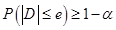 , in order to accept the model and consider it as sufficiently reliable for system prediction. Therefore, a model is exact, or with no bias (NB), when the differences (di) fit a normal distribution with mean zero.
Medina, Vargas-Villamil (4) indicate that CB is recognized by an average value of the differences ( ) distant from zero and that the graph of the points (zi, di=yi-zi) forms a horizontal band centered at with systematic distribution either positive or negative (points above and below the line
  ). When the samples are related, a t-test applied to determine if the mean of the differences is significantly different from zero, would prove the presence of CB in the model predictions.
Determination of proportional bias. PB is recognized in the graph of points (zi, di=yi-zi) whenever a positive or negative linear trend is found; the magnitude of the bias (di=yi-zi) increases or decreases in direct proportion to the predicted values (zi). A simple linear regression analysis of the bias vs predicted (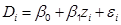 ) contributes to the detection of PB more objectively (2,8).
Validation of models with proportional bias. Given that we have PB, the points (zi, Di) i=1,2,…,n are related by 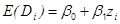 and
and 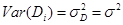 , with Di~
 . That is,
  , where
  ,
,  , and
, and  ~
~ , and thus, the model will be accurate when carrying out the correction
  . In practice, a regression model is fit and the errors (εi):
 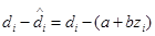 are estimated, where a and b are the least squares estimates of the intercept (β0) and the slope (β1), respectively. Thus, we would need only a statistical test for the required precision , which is translated to
  , once PB is removed by the referred correction.
If  ~
~ , then
 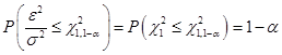 . Moreover, for e and α satisfying
 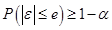 , it follows that
 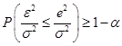 ; thus,
  and
and  where, in general,
  represents the quantile ( of the chi-square distribution with “k” degrees of freedom (
 ); that is,
 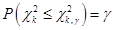 .
.
The indicated correction results in an accurate model, and only the statistical test for precision is needed. Thus, the following step is to test the hypotheses with the original proposal (OP) 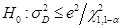 vs
vs 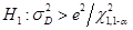 (3), or the alternative proposal (AP)
 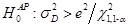 vs
vs 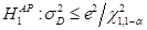 (8). The test statistic with ~
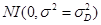 and under true null hypotheses
  or
or  is:
is:
 ~
~
or is rejected with a significance level α’ if  or
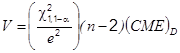
or  , where Vc corresponds to the calculated value of the test statistic (V), and (CME)D to the mean square of the error for the estimated model
  . Therefore, if is not rejected or is rejected, then the model is considered acceptable for prediction under OP and AP, respectively.
Another approach for evaluating precision once PB is corrected, is to use confidence intervals (CI), similar to the procedure presented by Medina et al 4 when the model has CB in its predictions. This approach is motivated by Freese’s proposal: different users of the model may have different requirements of precision, leading to different values of the maximum admitted error of the deviations (e).
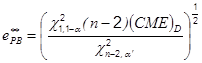
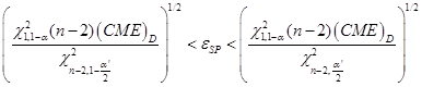
From the rejection region for , 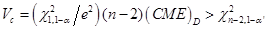 and solving for “e”, the critical error is found 8:
Therefore, will be rejected if  , and it will not be rejected if
  ; that is, if the model user specifies a value for “e” such that
  , then the model is considered acceptable in the prediction of the system under OP.
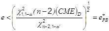
Using an analogous procedure for AP, the maximum anticipated error, or critical error was obtained (8):
Thus, if the model user specifies a value of “e” such that  , then the model is considered acceptable in predicting the system under AP. In a previous study (9), a hypothesis tests and confidence intervals are related, this relationship enables to construct one from the other.
Other published works from Reynolds (6) and Barrales et al (7) do not present the confidence interval (CI) for 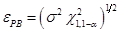 , the quantile 1-α of the distribution of
  (in practice, the errors (e) once PB is corrected) or equivalently
  , is the quantile 1-α of the distribution of
  since, if ~, then
 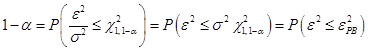 .
.
A (1-α’)100% CI for  8 based on CI (1-α’)100% for
  (where
 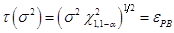 is an increasing monotonic function) is given by
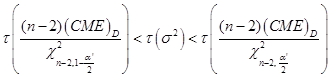
where  and
and  correspond to the critical errors
  and
and  , with the difference that α’ is substituted by α’/2. The estimated CI
  means that we have a confidence of 100(1-α’)% that the value of the distribution for
 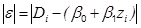 having below the 100(1-α) percent of the absolute errors is located in some location of the referred interval. This enables us to determine with certain probability an upper bound for the magnitude of the prediction error (e), and to use it in the evaluation of the evolution of the model for system prediction.
RESULTS
To illustrate the application of the methodology, the CI approach 4 was used with a published data set from Barrales et al 7, which corresponds to a model of grassland growth simulation. In this example, we applied the method of calculating the maximum anticipated errors or critical errors of the OP and AP, when the model has PB. In addition, 95% CI was calculated for , the 1-α quantile of the error (e) distribution, once PB is corrected with  .
.
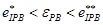
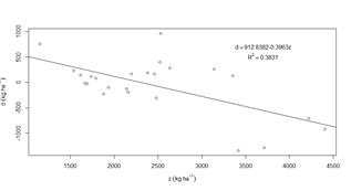
The distribution of the points in Figure 1 indicates that the model has PB in its predictions; the magnitude of the bias (di=yi-zi) decreases directly with the predicted values (zi) and the linear relationship was significant (d=912.838-0.396z: F=13.665, p=0.001). With α=α’=0.05, the critical errors were 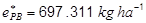 and
and  . Therefore, if the modeler or the model user specifies a value “e”
 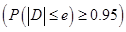 such that
  or
or  , then the model is considered sufficiently reliable in predicting the system based on OP and AP, respectively. For example, if e=1157 kg ha-1, the model is considered acceptable for predicting with both proposals (OP: e>697.311 kg ha-1; AP: e>1156.273 kg ha-1).
The 1-α’=95% CI for is  , and thus, we are 95% confident that the distribution value found below 1-α=95% of the absolute errors is located in some part of the interval (669.689 kg ha-1 - 1225.564 kg ha-1); that is, there is a 95% of probability that the magnitude of the prediction error does not surpass 1225.564 kg ha-1.
With 95% of confidence, the critical error with AP and CI for  would have to allow 1156.273 kg ha-1 as the minimum prediction error, which should not surpass 1225.564 kg ha-1. In this way, the validated model could be used to predict grassland growth. However, it would require a fit in its structure based on the presence PB in its predictions.
DISCUSSION
Identifying the type of bias may allow to improve the structure of the model and its evaluation, the data and methods used in all the processes of its construction, and validation 4. McCarthy et al have pointed out that testing a model helps to identify its weaknesses so that its predictive performance can be improved 10, since identification, and acceptance of inaccuracies of a model is a step towards the evolution of a more accurate, more reliable model 1.
The extensions we present for validating deterministic model possessing PB in their predictions are applied with no modifications in the model structure because this type of bias is removed from the available data (
zi, yi
) by means of the bias values (di), namely, by the correction .
The test statistic and critical error with AP require a larger maximum admissible error (e) value than that with OP, in order to infer whether the model is acceptable for predicting the system or not. A previous study by Medina et al 4 points out that the inconvenience of applying the OP is the ambiguity occurring when the null hypothesis is not rejected (H0) since what it can be inferred is that the data do not provide sufficient evidence to reject it, and that the affirmation stated in H0 is not accepted. Moreover, as the research hypothesis is posed in the alternative hypothesis, we recommend using the AP in validating a system prediction model.
Validation by means of critical errors or by the confidence limits approach (the latter being a procedure equivalent to the hypothesis testing approach, as mentioned above), is reduced to calculating the maximum anticipated error, or critical error, in which the model developer or the user decide whether the model is acceptable in predicting the system. This is carried out by comparing the critical error with the required accuracy (e) under the values α and α’ specified beforehand. This requires that the model developer or the user have good understanding of the system to establish, a priori, the maximum admissible error (e). Medina et al 4 recommend the CI approach to validate a model for several reasons. It provides the range of possible values of the parameter under consideration thus, it is more informative than hypothesis testing in the sense that it permits determining the a posteriori maximum admissible prediction error.
It should be pointed out that the critical error, or a posteriori maximum admissible error, can be used to compare several models for a single system, in such a way that the best model would be the one with the lowest critical error. To assess the improvement of a model in system prediction it is necessary to observe whether a posteriori maximum admissible error decreases at each process of improvement.
The estimated CI for the quantile 1-α of the error distribution, once PB is corrected, allows us to determine an upper bound for the magnitude of the prediction error with a certain probability, and to use it in the evaluation of the evolving model whenever an improvement is required. This is similar to the case of validating a model with CB in its predictions 4. Thus, based on the critical error with AP and the aforementioned CI, we can establish the minimum permitted prediction error, and what amount of error of prediction would not surpass.
In conclusion, the extensions to Freese’s statistical method presented here to validate models in the presence of proportional bias are applied without modification in the model structure.
In validating a model, we recommend using the confidence interval approach under the alternative proposal.
The confidence interval for the 1-α quantile of error distribution, once the proportional bias is corrected, allows determination of an upper bound for the magnitude of the prediction error.
Both a posteriori maximum admissible error, and the upper bound for the magnitude of the prediction error can be used to evaluate the evolution of a model in predicting the system in the face of a modification of the modeling process.

