The value of rural landscape in Aquitania (Colombia): application of spatial hedonic models in real estate analysis

El valor del entorno rural en Aquitania (Colombia): aplicación de modelos espaciales hedónicos en el análisis de bienes raíces

O valor do entorno rural em Aquitania (Colombia): aplicação de modelos espaciais hedónicos na análise dos nens de raiz

La valeur de l'entourage rural à la province d'Aquitania (Colombie) : application de modèles spéciaux Hédoniques dans l'analyse de biens immeubles

Ana Milena Plata Fajardo^*
Julio Cañón^**
Raffaele Lafortezza^***

^*Department of Forestry Engineering, Federal University of Paraná / Brazil. Email: aplatafa@gmail.com.
^**Universidad de Antioquia, Grupo GAIA, Medellín, Colombia. Email: jecanonb@gmail.com.
^***Department of Agricultural and Environmental Sciences, University of Bari, Italy. cgceo/Geography, Michigan State University, East Lansing, USA. Email: r.lafortezza@gmail.com.

Recibido: 2015-08-15 Aprobado: 2015-12-04 Disponible en línea: 2016-01-01

Como citar este artículo

Plata Fajardo, A. M., Cañón, J. y Lafortezza, R. (2015). The value of rural landscape in Aquitania (Colombia): application of spatial hedonic models in real estate analysis. Cuadernos de Desarrollo Rural, 12 (76), 155-179. http://dx.doi.org/10.11144/Javeriana.cdr12-76.vrla

Abstract

This study addresses the marginal economic value of environmental amenities, structural characteristics, neighborhood facilities, and accessibility on property in Aquitania - Colombia. Based on 400 assessed values of rural land property and on 21 characteristic variables of land amenities and facilities, the study compares three models: Ordinary Least Squares (ols), Spatial Lag Model (SLM), and Spatial Error Model (sem). Results show that both SLM and sem outperformed ols in identifying the significance of real estate attributes. Results shows that farmers value environmental amenities more than other attributes, being implicit the greater value of cattle over agriculture (onion) in land use. These models may help to support decisions in rural real estate economics.

Keywords: Akaike Information Criterion; Moran's I test; spatial hedonic price; spatial patterns

Resumen

El presente estudio aborda el valor económico marginal de las comodidades ambientales, características estructurales, instalaciones vecinas y la accesibilidad de las propiedades en Aquitania, Colombia. Tomando como base 400 valores calculados de propiedades de terreno rural y 21 variables características de las instalaciones y comodidades del terreno, este estudio compara tres modelos: Mínimos Cuadrados Ordinarios (ols), Modelo de Rezago Espacial (SLM) y Modelo de Error Espacial (SEM). Los resultados muestran que tanto el SLM como el sem superan al ols en la identificación de la importancia de los atributos de los bienes raíces. Los resultados muestran que los granjeros aprecian las comodidades del entorno sobre otros atributos, quedando implícito el mayor valor de la ganadería sobre la agricultura (cultivo de cebolla) en el uso del terreno. Estos modelos pueden ser de ayuda para sustentar decisiones respecto a la economía de los bienes raíces rurales.

Palabras clave: criterio de información de Akaike; prueba I de Moran; precio espacial hedónico; patrones espaciales

Resumo

O presente estudo trata do valor económico marginal das amenidades ambientais, características estruturais, instalações vizinhas e acessibilidade das propriedades em Aquitania, Colombia. Tomando como base 40c valores calculados de propriedades de terreno rural e 21 variáveis caraterísticas das instalações e amenidades do terreno, este estudo compara très modelos: Mínimos Quadrados Ordinários (ols), Modelos com Lag Espacial (SLM) e Modelos com Erro Espacial (SEM). Os resultados mostram que tanto o SLM quanto o sem superam o ols na identificação da importancia dos atributos dos bens de raiz. Os resultados mostram que os agricultores gostam do conforto do entorno sobre outros atributos, ficando implícito o maior valor da produção de gado sobre a agricultura (cultivo de cebola) no uso do terreno. Estes modelos podem ser de ajuda para suportar decisões no que diz respeito da economia dos bens de raiz rurais.

Palavras-chave: criterio de informação de Akaike; teste I de Moran; preço espacial hedónico; padrões espaciais

Résumé

La présente étude aborde la valeur économique marginale des commodités environnementales, caractéristiques structurales, installations proches et l'accessibilité des propriétés à la province d'Aquitania, Colombie. En prennent en tant que base 400 valeurs calcules de propriétés de terrain rural et 21 variables caractéristiques des installations et commodités du terrain, cette étude compare trois modèles : Modèle Carrés Ordinaires (ols), Modèle de Retarde de l'Espace, (SLM) et Modèle d'Erreur de l'Espace (SEM). Les résultats montrent que tantôt SLM que le sem dépassent au ols dans l'identification de l'importance des attributs de biens immeubles. Les résultats montrent que les fermiers apprécient les commodités de l'entourage sur les autres attributs, de ce fait il est implicite que l'élevage a une plus grande valeur par rapport à l'agriculture (planter de l'oignon) dans l'usage du terrain. Ces modèles peuvent ètre d'aide pour soutenir les choix par rapport à l'économie de biens immeubles ruraux

Mots clés: critère d'information de Akaike ; preuve I de Moran ; prix spécial hédonique ; patrons spéciaux

I. Introduction

Land price analysis is an important element of real estate economics (involving land and buildings in residential, commercial, and agricultural sectors), which is used by governments and the private sector in rural planning, and policy evaluation and implementation (Ismail, 2010).

While countries such as the United States, Switzerland, and Taiwan have been developing systems of rural real estate ownership to manage and guarantee property information and to identify the attributes of properties (Hoesli & MacGregor, 2000), in developing countries, by contrast, information concerning rural real estate is scarce and not easily available. Citizens and rural owners are often informed about land prices through annual news reports, but there is no systematic collection of information about the attributes of rural property.

Rural land is usually valued for its productivity-bearing attributes, such as: environmental amenities, neighborhood facilities, accessibility, and structural characteristics. Hedonic analysis investigates the existence of these attributes and how they interact to determine the price that people are willing to pay for a land unit (Coulson, 2008). Hedonic Price Modeling (hpm) is a useful econometric tool to analyze the price of a heterogeneous good, and has been widely used to value housing attributes and to construct price indices, particularly related to real estate and land (Malpezzi, 2003). hpm is appropriate to empirically measure the value of externalities that are, by definition, not separately transacted on the market (not sellable on their own). However, the non-existence of a separate market for externalities does not prevent them from being internalized or priced, since externalities can be traded jointly with other goods (Chau et al., 2004).

Even though hpm seems to be the best way to observe the influence of the attribute on the price of rural land, several authors have been refuting certain assumptions of this approach. hpm, for instance, only works under the assumption of market equilibrium and does not deal with the interrelationships between the implicit prices of the attributes (Dusse & Jones, 1998). hpm based on Ordinary Least Squares (ols), for instance, violates two basic assumptions: i) that model residuals are uncorrelated with each other (no autocorrelation), and ii) that they have constant variance (homoscedasticity). The existence of spatial autocorrelation and heterogeneity in modeling housing datasets will reduce the efficiency of the regression and mislead the interpretation of the ols model results (Hamilton, 1992).

In most hedonic specifications, coefficients of housing attributes are held constant under the assumption that each attribute has a unique marginal price throughout the entire market area (Xu, 2008). However, there is increasing evidence that marginal prices of some key housing attributes vary according to particular systematic patterns. Xu (2008) provides strong evidence that the marginal prices of key housing attributes are not constant, but vary with household profile and absolute-location context.

The issues of heterogeneity and autocorrelation prevent ols from representing the varying relationships over rural land. To tackle this concern, Paez et al. (2007) posit that urban housing markets should be organized into a series of submarkets, each of them represented by a unique functional relationship between prices and property attributes. Following this approach, identifying the attributes contained in a parcel of rural land can shed light on the causes of land use segregation. In this way, market segregation may be determined by the patterns of the attributes contained in the property.

In most land use segregation models —the expansion method in Can and Megbolugbe (1997) and Theriaut et al. (2003), and the geographically weighed regression in Bitter and Gordon (2007)— the marginal prices are usually related to spatial variables such as neighborhood and accessibility characteristics. In this regard, Anselin (1998, p. 7) points out the use of spatial econometrics as the collection of techniques that deal with the peculiarities caused by space in the statistical analysis of regional science models. With emerging technology associated with gis as well as progress in the fields of spatial econometrics and statistics, several researchers (Anselin et al., 2000; Bastian et al., 2002; Pace et al., 2004) have explored the spatial nature of housing within the hedonic analysis. According to Hoesli and MacGregor (2000, p. 64), hedonic estimation has clearly matured over the past three decades, from being a novel mathematical tool to becoming the standard way economists deal with housing heterogeneity.

Spatial econometrics explicitly accounts for spatial autocorrelation (Zhang & Hickel, 2004) and spatial heterogeneity in real estate (Patton & McErlean, 2003; Can, 1997; Li et al., 1994), spatial autocorrelation being a weaker expression for spatial dependence (Wilhelmsson, 2002). Two types of spatial dependence are usually considered to fit spatial models (Ward & Gleditsch, 2008): Spatial Lag Models (SLM) and Spatial Error Models (sem).

Our study focuses on the application of spatial hpm in rural regions with scarce public information about properties. In this study, and in accordance with Li et al. (1994), we consider rural real estate as a bundle of heterogeneous housing attributes rather than as a single-valued commodity. gis tools and spatial statistics were used to map the spatial structure of rural land attributes and to determine the significance of this structure in the price of rural land properties. Research included the field identification of 21 attributes that could affect the price of 400 rural properties in a Colombian municipality (Aquitania) devoted mainly to agriculture and cattle.

We compare the application of three hpms (ols, SLM, and sem) to estimate owners' willingness to pay for four categories: i) environmental amenities, ii) neighborhood facilities, iii) structural characteristics, and iv) accessibility.

This work initially describes the study site, the methodology employed in the identification of the attributes, and the application of the three hpms. The results of ols, SLM, and sem are presented, followed by a discussion on their applicability and meaning. Finally, some conclusive remarks highlight the benefits of applying spatial hpm in areas with little available information.

2. Methodology

2.1 Study area

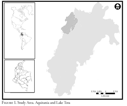
The study area encompasses the rural land of Aquitania, a Colombian municipality of 945 km² and 20,454 inhabitants (15,619 in the rural area and 4,855 in the municipal town) located on the east side of Lake Tota, the country's largest natural lake in the Eastern Andean Cordillera (Figure 1 the blue shaded area represents Tota Lake and the gray area represents Aquitania Municipality). Aquitania has a long established history of agricultural practices mostly devoted to producing onion, of which it is the main supplier in the country. Aquitania strategically connects the capital city of Bogota to the eastern Casanare region, and from there to Venezuela and South America. Despite its long history (the municipality was founded in 1777), strategic location, and wide range of environmental resources, the municipality registers very poor indices of human development (0.597) and educative coverage (45%) (Gobernación de Boyacá, 2012), which in turn reflect the low level of entrepreneurship in the region.

Some environmental amenities (i.e., water availability, land use, and flood hazards) of the municipalities within the Lake Tota basin have been studied by some authors (Pedraza, 2005; Ricaurte, 2005; Vergara, 1988). Ricaurte (2005), in particular, identified the main problems and conflicts related to water uses among several stakeholders. Aquitania is responsible for nearly 95% of the production of onion in Colombia. Farmland occupied by irrigated onion crops accounts for 4,500 hectares and demands about 91% of the water used within the basin (Gobernación de Boyacá, 2012).

2.2. Information sources

Three different sources of information were employed in this study. The primary source was derived from the municipality of Aquitania's office of treasury, which every year collects the prices of rural and urban land, and announces the value of all properties in the municipality (these values are used for rural and urban planning, and for tax purposes). The definitions of all environmental amenities, accessibility, and road quality variables were obtained from the governmental agency in charge of geographical data (Instituto Geográfico Agustín Codazzi [IGAC]) and processed in ArcGiS®. Lastly, the information regarding neighborhood facilities and structural characteristics was directly surveyed and geographically coded using Arcmap®. Two variables were collected for accessibility measurements: the coordinates (latitude and longitude) of the centroids of the lake and market districts (CMD), and the measured distances of each rural parcel to the lake and the CMD. The data were verified for quality and converted into formats suitable for further analysis. In this stage, all the hedonic variables (including GiS-constructed spatial variables) were defined, and the spatial weight matrix needed for spatial hedonic modeling was established. The final hedonic datasets contain 400 assessed values as the dependent variable and 21 independent variables.

2.3. Data processing

gis was applied to real estate in the residential, commercial, and rural sectors (Ismail, 2010) as a relevant tool for housing market analysis, given that all residential real estate information is inherently related to a spatial reference (Belsky et al., 1998). gis has the advantages of efficient data integration and spatial analysis (Imar & Hamid, 2002). For example, Tota Lake Basin (tlb) is a socio-economic heterogeneous area with four main land uses identified in the gis: Onion, Mixed Farming, Cattle, and Forestry. If properly designed, gis maps can help analysts to detect patterns in data and spatial relationships between two or more phenomena (Pisati, 2012). When analyzing spatial point patterns, it is of interest to determine whether the observed data points exhibit some form of clustering. In general, spatial autocorrelation implies spatial clustering, i.e., the existence of sub-areas of the study area where the attribute of interest (Y) assumes higher than average values (hot spots) or lower than average values (cold spots). Figure 2 shows the location of attributes and land use segregation in the study area. A distinct spatial pattern is distinguishable, with the highest concentration of onion land use near the lake and of cattle land use far from the lake (onion and cattle are the land uses with the highest rural parcel prices in the municipality).

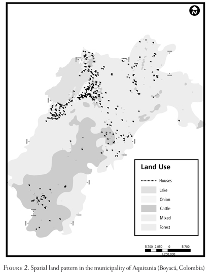
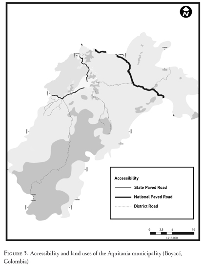
Figure 3 shows the spatial pattern of accessibility of the Aquitania municipality. In a spatial context, there is evidence of heterogeneity for this variable. Paved roads, for instance, are located to the north and near the lake (where onion crops are planted), whereas district roads are located to the south of the municipality (where the main land use is cattle breeding). Although onion croplands are more easily accessible, the price of rural parcels for cattle breeding does not seem to be affected by road conditions.

2.4. Hedonic Price Modeling

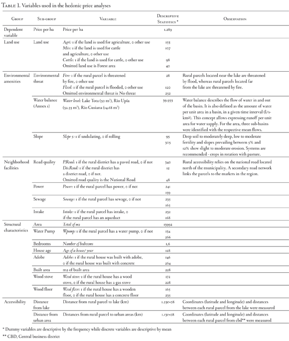
hpm establishes a regression of property transaction prices against the corresponding property characteristics (Fletcher et al., 2000). Since there is no information avai lable for transaction price, assessed property prices were used. Assessed prices were obtained from the treasury of the municipality. Seven groups of data were gathered for this study: Rural Parcel Price, Parcel Location (X and Y coordinates), Land Use, Environmental Amenities, Neighborhood Facilities, Accessibility, and Structural Characteristics. The explanatory variables are the attributes involved in the rural parcel. Table i summarizes the 21 variables collected, their definition, and some observations.

2.4.1. The ols Model

The ols model considered in this study is expressed as follows:

RPP = β₀ β₁ LU + β₂ EA + β₃ NF + β₄ SC + β₅ A + ε (I)

Where rpp is Rural Parcel Properties; lu refers to Land Use; ea are the Environmental Amenities; nf are the Neighborhood Facilities; sc are the Structural Characteristics; and A is Accessibility. In this study, a linear functional form is favored over a semi-logarithmic form because the semi-log functional form may have potential undesirable effects on the transformed residuals, obscuring the original spatial pattern, and subsequently affecting the measurements of spatial autocorrelation or the construction of variance-covariance structures (Bowen et al, 2001). Spatial models are generally specified as linear regression models with spatial interdependence taking the form of a linear additive relationship of observations on neighbours (Wilhelmsson, 2002a, p. 95).

2.4.2. Spatial models

2.4.2.1. Spatial Weights Matrix

Before running a spatial model, it is necessary to create a Spatial Weights Matrix. Most spatial data analyses require an explicit definition of the degree of proximity among the objects of interest. Typically, the degree of spatial proximity among a given set of N objects is represented by an N N matrix called Spatial Weights Matrix and denoted by W (Pisati, 2012). By convention, the diagonal elements of W are set to zero and the off-diagonal elements are normalized to sum one in each row. W quantifies the spatial relationships that exist among the features in a dataset. While the format of W may vary, the concept is simply expressed in a table with one row and one column for each feature in the dataset. The cell value for any given row/column combination is the weight that quantifies the spatial relationship between those row and column features (esri, 2013). Each element of W, which is denoted by W_ij, expresses the degree of spatial proximity between the pair of objects i and j.

2.4.2.2. Spatial Lag Model (SLM)

The SLM (spatial autoregressive process in the outcome variable) considers the spatial autocorrelation of land value (i.e., each land parcel depends partially on the characteristics of its neighboring parcels). The SLM is used to correct the hedonic price estimates from spatial effects. The functional formula of the SLM is:

RPP = α + Xβ + Lβ1 + Nβ2 + Eβ3 + Sβ4 + Aβ5 + pWp + ε

Where Wp is the spatially lagged dependent variable; is the spatial autocorrelated parameter; is a constant; is a vector of coefficients for the independent variables; and is a vector of the independent and identically distributed error.

2.4.2.3. Spatial Error Model (SEM)

The sem (spatial autoregressive process in the error term) incorporates the residual from a hedonic regression as the explanatory variable in a structural equation model. The model takes into account the spatial dependence through the error term, as presented in the following formula:

RPP = α + Xβ + Lβ + Nβ + Eβ + Sβ + Aβ + u (3)

U = λWu + ε

Where L is a coefficient of the spatially correlated error and Wu is the spatially lagged error term.

2.5. Comparisons among models

The results of the ols, SLM, and sem were tested for spatial dependence using Moran's I test (Pisati, 2001), which provides a measure of the spatial correlation between neighbors. Test values range from -1 for perfect dispersion to +1 for perfect correlation, with 0 indicating a random spatial pattern (Linderhof et al., 2007). Moran's I tests the null hypothesis of no spatial effects in the outcome variable and requires the creation of a weights matrix. There is no explicit advice regarding the specification of the neighboring structure and types of weights (Dubin, 1998). A common method for creating a weights matrix is by employing distance bands; a fixed distance band is the default conceptualization of spatial relationships. Inverse-distance matrices are a common parameterization for the spatial weights matrix. The bands were calculated with Stata® based on the exact location of each house and parcel centroids ensuring that all observations had at least one neighbor. The definition of a neighbor includes observations within an area of 55,800 m² (5.58 ha), which represents the average distance between centroids.

Alternatively, the Breusch-Pagan-Lagrange Multiplier tests the null hypothesis that the error variances are all equal versus the alternative that the error variances are a multiplicative function of one or more variables (Zhang & Hickel, 2004). The models in our study were also tested using two main variants of the Breusch-Pagan tests: the lm-lag and the lm-error. The lm-lag tests the null hypothesis of no spatial autocorrelation in the dependent variable. The lm-error tests the null hypothesis of no significant spatial error autocorrelation (Ismail, 2010). These two tests provide a basis for choosing an appropriate spatial regression model (Anselin, 1997). Significance of lm-error points to a spatial error model, while significance of lm-lag points to a spatial lag model.

Models were also compared using the Akaike Information Criterion (AIC), which provides a relatively simple method for determining the best model performance. The value of the aic may be used as a descriptive measure of overall model performance when judging non-nested models (Osland, 2010). A lower aic value indicates a closer approximation of the model to reality (Wang et al., 2005). Thus, in this study, a spatial model is considered to be significantly improved from its corresponding ols model if the aic values of the spatial lag and spatial error are lower than those of the ols, and the F-test is significant at a 0.05 confidence level. To compare the ability to deal with spatial autocorrelation, global Moran's I values were calculated for the residuals from the ols and spatial models.

3. Results

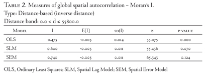
The models described above were designed to emphasize different spatial processes. This study carried out a regression for each spatial process using neighboring observations. A spatial autocorrelation approach may partially eliminate spatial dependence by calibrating models within a local and more homogeneous context. In general, a house price is related to the characteristics of the house and property itself and those of the neighborhood and community, the environmental amenities, and accessibility measures. Nevertheless, six variables were not significant: two refer to structural characteristics (bedrooms and house age), two concern neighborhood characteristics (paved road and district road), and one refers to accessibility measures (distance from urban center). According to Moran's I test, spatial regression models are necessary to improve the efficiency and consistency of the predictors. The results comparing Moran's I statistics on the residuals from OLS and the two models are shown in Table 2. Significant, positive spatial autocorrelations were found in the OLS model (Moran's I = 0.473, p = 0.00). This result indicates that the OLS model is unsuitable for identifying the relationships between Rural Parcel Price and its environmental amenities. Although SLM and SEM also show a high Z score, their p value statistics reject the null hypothesis of autocorrelation.

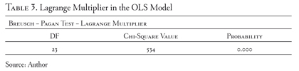
Results of the Breusch - Pagan test are shown in Table 3. The highly significant Chi-square value (534), suggests the presence of heteroskedasticity, therefore, the error variances increase as the predicted values of rural land price increase.

The results in table 4 indicate the existence of a greater spatial autocorrelation in the Spatial Error Model than in the Spatial Lag Model.

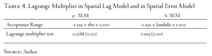
Given the normalization of the spatial-weighting matrix, the parameter space for p and X is taken to be the interval (-1.332, - 1) (Kelejian & Prucha, 2010). The estimate of X is positive, large, and significant, indicating strong spatial-autoregressive dependence in the error. In other words, the rural land prices in a county are strongly affected by prices in the neighboring counties. This effect may be explained by a "coordinated" decision on prices among property owners based on a common knowledge about selling prices (Kelejian & Prucha, 2010).

The aic parameter estimation and goodness-of-fit are listed in Table 5. The aic decreases in both spatial models relative to the ols model (from 4651 to -544.9 in the sem and to -468.9 in the SLM), which suggests an improvement of the goodness-of-fit for the spatial error specification. SLM and sem improve the reliabilities of the relationships by reducing the spatial autocorrelations in residuals (in fact, the SLM and sem residuals have no significant spatial autocorrelation).

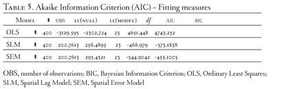
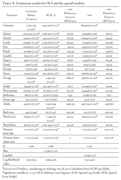
Table 6 presents a set of statistics comparing the performance of the two spatial models with the ols model. Although the three models exhibit a > 95% variation in rural parcel price (which suggests that the variables collected have an acceptable goodness-of-fit in the three models), the presence of autocorrelation in the ols model indicates a spatial bias that invalidates its results. Although both spatial models reach high R² values, have parameter estimates of the same sign, and are of similar magnitude, the SLM results in slightly more variables being statistically significant at the 5% level of significance and having a better aic than sem score.

4. Model validation

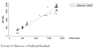
Validation is the task of demonstrating that the model is a reasonable representation of the actual system: it reproduces the system's behavior with enough fidelity to satisfy analysis objectives (Ahmad, 2013). Numerous statistical tools exist for carrying out model validation, but the primary tool for most process modeling applications is graphical residual analysis. Graphical methods have an advantage over numerical methods for model validation because they readily illustrate a broad range of complex aspects of the relationship between the model and the data (Stoimenova, 2003).

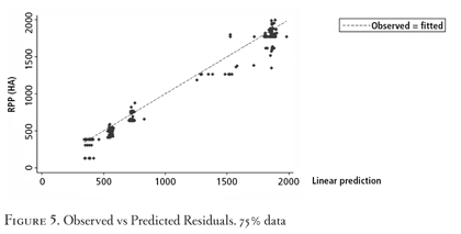
Figure 4 illustrates the residuals from the observer model and the predicted model. To validate the model, the slope and intercept parameters were compared against the 1:1 line. The graph shows that the regression of predicted (y-axis) vs. observed data (x-axis) behaves well. This process was repeated once again deleting 15% of the data to determine whether the plot has the same behavior (Figure 5). The figures show that the models fit the data, and that the residuals approximate the random errors that establish a statistical relationship between the explanatory variables and the response variable.

These results are similar to those found by Gao et al. (2002), who point out the need of a cross-validation approach to see how well the prices already being observed can be predicted with a portion of the same dataset. An application of a similar method can be seen in Bourassa et al. (2001), where 80% random samples are modeled to predict the remaining 20% samples, using the sum of squared errors as a criterion to evaluate the proposed model.

Gao et al. (2002) also address the distribution of observations and predictions by a scatter plot of observed unit prices vs. predicted unit prices. The range occupied by the scatter points indicates the prediction power of a model. All points being on a 45^o diagonal line indicates a perfect prediction, and higher prediction power is suggested by how narrow the range is to the 45° line.

5. Discussion

One potential objection to both the SLM and sem is that their parameters are not identified (Anselin et al., 2008). However, according to Elhorst (2011), the results should be similar to those of the "original" parameter estimates (Elhorst, 2011). Columns 4 and 6 of Table 6 report the marginal effect of each variable on house price in the SLM and sem. The marginal effect represents the differential variation in house price due to a unit change in the amount of the evaluated attribute (Osland, 2010).

All the environmental characteristics and land uses appear to be statistically significant in the OLS and spatial models, suggesting that those attributes are important determinants of rural parcel price. The estimated results suggest that in regard to land use, onion represents the highest influence on rural parcel price, since land uses for onion increase the rural parcel price by 852.81/ha, other variables remaining constant (prices are in dollars, considering an exchange rate of 1900 Colombian Pesos [cop]/dollar). Three of five variables (i.e., power, sewage, and intake) from neighborhood facilities are statistically significant and have the expected increasing impact on marginal price. Although number of bedrooms, house age, and built area are common significant variables in HPMs, this is not the case for rural parcel price in Aquitania. In this sense, landowners value environmental resources more than structural characteristics, since the land is mostly dedicated to productive (agriculture, cattle, forest, and tourism) rather than residential activities. Results from the empirical model suggest that rural parcel price in the presence of fire threat is lower than in the presence of a flood threat. As expected, rural parcels in undulating slopes are US$ 88.58 more expensive than rural parcels in rolling slopes. This finding demonstrates that farmers value environmental amenities more that structural characteristics, neighborhood attributes, and accessibility except for the variable sewage, which appears to have a higher positive impact than land uses on rural parcel price. However, a more detailed examination of the data indicates that only few rural parcels have sewage and that these are devoted to tourism.

The results further demonstrate that the coefficient of the accessibility variable is not significant at a 95% confidence level, which implies that, contrary to expectation, the location near the lake does not impact the price of rural parcels. The reason why the variable accessibility is not significant can be seen in Figure 2. The map shows the highest rural parcel price for onion and cattle uses. These properties are distant from each other, with the national road being close to the onion parcels; yet, it seems that distance does not affect the price of rural parcels. The rural transportation network is an important issue in rural parcel pricing which, however, does not rely solely on road quality but also on the productivity sector.

According to hazard maps provided by igac (2008), Aquitania has been historically threatened by forest fires and floods. This was the main reason for including their effects in the rural parcel price. Results indicate that fires reduce the price of a parcel by $US 992/ha, while floods reduce the price only by $US 474/ha. This major reduction in marginal price due to fires could be associated to cheaper parcels near forested areas, which are not as economically profitable for agrobusinesses as are parcels of onion production and cattle breeding. Floods, on the other hand, are sometimes necessary for onion production in the agricultural land near the lake, which can explain the lower marginal effect compared to fire threats.

6. Conclusive remarks

Research on the significant attributes that impact rural parcel prices is essential to understand how owners and potential buyers value rural estate as an investment or a consumption decision, especially in cases where no explicit data exist to determine such values. This is particularly important in countries like Colombia, where the official real estate system is not well developed, i.e., the government holds some basic information on transaction price, area, address, and identification number of the owner, but even this limited data is either held confidential or not publicly available.

In this regard, our study demonstrates the applicability of spatial econometric models that include lags of the dependent variable to describe the value of rural land associated with several attributes in data-limited regions. The SLM and sem outperformed the traditional ols approach based on Moran's I test and the Akaike Information Criterion by describing relational variables that are dependent on location. This is particularly important because it shows that the models are capable of discerning the differential impact of the attributes, even indicating situations contrary to common sense expectations. For instance, the spatial mapping in Aquitania shows two discrete clusters in land use: one for parcels dedicated to agriculture (close to Lake Tota) and the other for parcels mainly devoted to cattle breeding (towards the Southwest). The first cluster also benefits from better access to national roads, whereas the second cluster relies more on access to secondary roads and requires long traveling distances to reach regional markets. Contrary to the expected high impact that this asymmetry in accessibility should have on the value of rural land, the spatial models indicate that it is not as relevant for owners and buyers as other attributes associated with structural characteristics (i.e., the negative marginal effect of houses built with adobe), neighborhood facilities (i.e., the positive marginal effect of access to sewage), or environmental amenities (i.e., the negative marginal effect of proximity to a flood-prone or fire-prone area). An explanation to this finding may depend on historical and cultural aspects, since owners are long established and buyers may belong to the same region and share similar expectations on mobility due to the common precarious road infrastructure, which is seen as part of "everyday life".

The use of these modeling approaches, even in the absence of sound databases, is beneficial for private and public sectors, in general. They provide a different outlook of the attributes most valued by people in a local context, detecting patterns in data and spatial relationships that may serve as a basis to organize, present, and interpret information in a way that is most efficient and economical.

Acknowledgements

The first author received funding from the Latin American and Caribbean Environmental Economics Program (LACEEP) through its Small Grants Program for Research in Environmental Economics. The second author was partially funded through the usaid-nsf peer Cycle 1 Project 31: impacts of climate change on tropical wetlands: tracking the evolution of two Andean lakes and a floodplain cienaga in Colombia. The authors thank Professor Fabio Vélez at Universidad de Antioquia for his help in developing first versions of the GIS maps.

References

Ahmad, T. (2013). Modeling and Control of Dialysis Systems: Volume 2: "Biofeedback Systems and Soft Computing Techniques of Dialysis". doi: 10.1007/978-3-64227558-6.         [ Links ]

Anselin, L. (1998). gis Research Infrastructure for Spatial analysis of Real Estate Markets. Journal of Housing Research, 9 (1), 113-133.         [ Links ]

Anselin, L., Varga, A., & Acs, Z. J. (2000). Geographic and Sectoral Characteristics of Academic Knowledge Externalities. Papers in Regional Science, 79 (4), 435-443.         [ Links ]

Anselin L., Le Gallo J. & Jayet, H. (2008). Spatial panel econometrics. In L. Mätyäs & P. Sevestre (Eds.), The econometrics of panel data, fundamentals and recent developments in theory and practice (3^rd ed., pp 627-662). Dordrecht, The Netherlands: Kluwer Academic Publishers.         [ Links ]

Bastian, C. T., Mcleod, D. M., Germino, M. J., Reiners, W. A., & Blasko, B. J. (2002). Environmental Amenities and Agricultural Land Values: A Hedonic Model Using Geographic Information Systems Data. Ecological Economics, 40 (3), 337-349.         [ Links ]

Belsky, E., Can, A. T., & Megbolugbe, I. F. (1998). A Primer on Geographic Information Systems in Mortgage Finance. Journal of Housing Research, 9 (1), 5-31.         [ Links ]

Bitter, C., & Gordon, F. (2007). Incorporating spatial variation in Housing Attribute Prices: A Comparison of geographically weighted regression and the Spatial Expansion Method. Journal of Geographical Systems, (9), 7-27.         [ Links ]

Bowen, W M., Mikelbank, B. A., & Prestegaard, D. M. (2001). Theoretical and Empirical Consideration Regarding Space in Hedonic Housing Price Model Application. Growth and Change, 32 (4), 466-490.         [ Links ]

Can, A. T., & Megbolugbe, I. F. (1997). Spatial Dependence and House Price Index Construction. Journal of Real Estate Finance and Economics, (14), 203-222.         [ Links ]

Chau, K. W, Yiu, C. Y., Wong, S. K., & Wai-Chung Lai, L. (2004). Hedonic Price Modelling of Environmental Attributes: A Review of the Literature and a Hong Kong Case Study. Welfare Economics and Sustainable Development, 2.         [ Links ]

Coulson, E. (2008). Chapter 1: An Introduction and Discussion of Origins. In A. Baranzini, J. Ramirez, C. Schaerer & P. Thalmann (Eds.), Hedonic Methods in Housing Markets: Pricing Environmental Amenities and Segregation. Springer Science & Business Media.         [ Links ]

Dubin, R. (1998). Spatial Autocorrelation: A Primer. Journal of Housing Economics, (7), 304-327.         [ Links ]

Dusse, N., & Jones, C. (1998). A Hedonic Price Model of Office Rent. Journal of Property Valuations and Investment, 16 (3), 297-312.         [ Links ]

Elhorst, J. P. (2011). Spatial Panel Models. University of Groningen, Department of Economics, Econometrics and Finance.         [ Links ]

Environmental Systems Research Institute (esri) (2013). Spatial Statistics Toolbox. Retrieved on July 29, 2013, from http://resources.esri.eom/help/9.3/arcgisdesktop/com/gp_toolref/spatial_statistics_toolbox/spatial_weights.htm.         [ Links ]

Fletcher, M., Gallimore, P., & Mangan, J. (2000). The Modelling of Housing Submarkets. Journal of Property Investment & Finance, 18 (4), 473-487.         [ Links ]

Gao, X., Asami, Y., & Chung, C. (2002). An Empirical Evaluation of Hedonic Regression Models. csis Discussion Paper n^o 46 Gobernación de Boyacá (2012). Plan Departamental de Desarrollo 2012-2015 (Original in Spanish).         [ Links ]

Hamilton, J. D. (1992). Time Series Analysis. Princeton, N.J.: Princeton University Press.         [ Links ]

Hoesli, M., & Macgregor, B. D. (2000). Property Investment Principles and Practice of Portfolio Management. Harlow: Longman. Instituto Geográfico Agustín Codazzi (igac) 2008. Cartography of Aquitania, 1: 250.000 (Original in Spanish).         [ Links ]

Imar, M., & Hamid, A. M. (2002). Incorporating a Geographic Information System in Hedonic Modelling of Farm Property Values. Lincoln University.         [ Links ]

Ismail, S. (2010). Hedonic Modeling of Housing Markets Using Geographical Information System (gis) and Spatial Statistics: A Case Study of Glasgow, Scotland. Universiti Teknologi Malaysia.         [ Links ]

Kelejian, H. H., & Prucha, I. R. (2010). Specification and Estimation of Spatial Autoregressive Models with Autoregressive and Heteroscedastic Disturbances. Journal of Econometrics.         [ Links ]

Forthcoming Li, H., & Reynolds, J. F. (1994). A simulation experiment to Quantify Spatial Heterogeneity in Categorical Maps. Ecology, (75), 2446-2455.         [ Links ]

Linderhof, V, Nowicki, P., Leeuwen, E., Reinhard, S., & Smith, M. (2007). Manual for the tests of spatial econometric model. Research report, The Hague: lei, part of Wageningen ur, 2011 (spard Deliverable D4. 1).         [ Links ]

Malpezzi, S. (2003). Hedonic Pricing Models: A Selective and Applied Review. In T. O'Sullivan, & K. Gibb (Eds.), Housing Economics & Public Policy. Oxford: Blackwell Publishing.         [ Links ]

Osland, L. (2010). An Application of Spatial Econometrics in Relation to Hedonic House Price Modeling. Journal of Real Estate Research, 32 (3), 289-320.         [ Links ]

Pace, R. K., & Lesage, J. P. (2004). Spatial Econometrics and Real Estate. Norwell, MA: Kluwer Academic Publishers. Issued as: Journal of Real Estate Finance and Economics, 29 (2).         [ Links ]

Paez, A., Long, F., & Farber, S. (2007). Moving Window Approaches for Hedonic Price Estimation: An Empirical Comparison of Modeling Techniques. Centre for Spatial Analysis/School of Geography and Earth Sciences. McMaster University.         [ Links ]

Pedraza, J. (2005). Reglamentación de las aguas derivadas del lago de Tota a través del túnel de Cuitiva. In Corpoboyaca-puj (Org.), Plan de Ordenación y Manejo Integrado del Lago de Tota.         [ Links ]

Pisati, M. (2001). Tools for Spatial Data Analysis. Stata Technical Bulletin 60: 2137. Stata Technical Bulletin Reprints, 10 (277). College Station, TX: Stata Press.         [ Links ]

Pisati, M. (2012). Spatial Data Analysis in Stata an Overview. Department of Sociology and Social Research, University of Milano-Bicocca (Italy).         [ Links ]

Ricaurte, P. (2005). Problemática ambiental. In Corpoboyaca-puj (Org.), Plan de Ordenación y Manejo Integrado del Lago de Tota.         [ Links ]

Stoimenova, E., Datcheva, M., & Schanz, T. (2003). Statistical Modeling of the Soil Water Characteristic Curve for Geotechnical Data. In Proceedings of the First International Conference for Mathematics and Informatics for Industry (pp. 356-366).         [ Links ]

Thériaut, M., Des, R. F., Villeneuve, P., & Kestens, Y (2003). Modelling Interactions of Location with Specific Value of Housing Attributes. Property Management, (21), 25-48.         [ Links ]

Vergara, I. (1988). Investigación hidrogeológica de la cuenca del lago de Tota. In I. Vergara, Estudio de crecientes y modelo de operación del lago de Tota (vol. II).         [ Links ]

Wang, Q., Ni, J., & Tenhunen, J. Q.J (2005). Application of a Geographically-Weighted Regression Analysis to Estimate Net Primary Production of Chinese Forest Ecosystems. Global Ecology and Biogeography, 14 (4), 379-393.         [ Links ]

Ward, M. D., & Gleditsch, K. S. (2008). Spatial Regression Models. Thousand Oaks, CA: Sage.         [ Links ]

Wilhelmsson, M. (2002). Spatial Model in Real Estate Economics. Housing Theory and Society, (19), 92-101.         [ Links ]

Xu, T. (2008). Heterogeneity in Housing Attribute Prices: An Interaction Approach between Housing Attributes, Absolute Location and Household Characteristics. City Futures Research Centre, The Faculty of Built Environment, University of New South Wales, Australia.         [ Links ]

Zhang, L., & Hickel, K. (2004). Water Balance Modelling over Variable Time Scales Q Shao, CSIRO Land and Water, CSIRO Mathematical and Information Sciences.         [ Links ]