ARTÍCULO CIENTÍFICO / RESEARCH ARTICLE

Pedro Mario Wightman R.^{* 1}, Miguel A. Labrador^{** 2}

1 Universidad del Norte (Colombia)

2 Universidad del Sur de la Florida (Estados Unidos)

* Ingeniero de Sistemas, Ph. D. Profesor asistente, Universidad del Norte, Barranquilla, Colombia. pwightman@uninorte.edu.co

Correspondencia: Universidad del Norte, km 5 vía a Puerto Colombia, A.A. 1569, Barranquilla (Colombia). Tel: 3509-509, Ext. 4268.

** Ingeniero Electrónico, Ph. D. Profesor asociado, University of South Florida, Tampa, Florida, USA. mlabrador@usf.edu

Fecha de recepción: 30 de junio de 2010
Fecha de aceptación: 1 de octubre de 2010

Resumen

Control de Topología-(CT) es una estrategia para ahorrar energía en las redes inalámbricas de sensores. Construcción de Topología-(CnT) es el área de CT que estudia la reducción de la topología de la red, manteniendo características como cubrimiento y conectividad. Las dos principales estrategias existentes para CnT se basan en reducir la potencia de transmisión de los nodos, como el KNEIGH-Tree, o en disminuir el número de nodos activos, como A3 y A3Cov. Ambas estrategias reducen el consumo de energía en la red, extendiendo su vida útil; sin embargo, hasta ahora estas estrategias no se han comparado entre ellas. Este artículo evalúa los tres protocolos mencionados en términos de su impacto en la vida de la red y la cobertura de área. Los resultados en redes densas muestran que A3 y A3Cov superan en más de 100% los resultados de KNEIGH-Tree.

Palabras clave: Construcción de topología, control de topología, cubrimiento de área, conectividad de red, atarraya, KNEIGH.

Abstract

Topology control-TC is a strategy used to save energy in wireless sensor networks. Topology construction-TCn is the area of TC that studies the reduction of the network topology, while maintaining characteristics like connectivity and coverage. There are two main strategies to reduce the topology of a network: reducing the transmission power, like the KNEIGH-Tree, and decreasing the number of active nodes in the network, like A3 and A3Cov. Both strategies reduce the energy consumption and, therefore, increase the network lifetime; however, these strategies have not been compared against one another. This paper compares the three protocols mentioned before in terms of the network lifetime and coverage. The results show that in dense networks, the A3 and A3Cov protocols extend the lifetime of the network more than twice than that of the offered by the KNEIGH-Tree protocol.

Keywords: Topology Construction, Topology Control, Area Coverage, Network Connectivity, Atarraya, KNEIGH.

During the past decade, Wireless Sensor Networks (WSNs) have received increased interest from the scientific community. Thanks to important developments in microelectronics, radio devices and low-power electronics, WSN technology is being developed and deployed in many scenarios in which pervasive monitoring is necessary but cannot be done in person due to lack of resources, time or because the location or conditions represent danger to the individuals.

Even today, one of the biggest constraints of WSNs is their energy consumption: most of the existing devices work with regular batteries which limit their lifetime considerably. This fact must be taken into account by the network designers in order to include energy-efficient and energy-aware protocols in order to reduce the rate of energy consumption in the network and extend the network lifetime.

Topology Control (TC) is one of the most well known strategies for saving energy in the network. The main objective of this technique is to reduce the network topology, number of active links and active nodes, while maintaining connectivity of the nodes and coverage of the area. TC considers two main processes: Topology Construction (TCn), which is in charge of reducing the initial topology, and Topology Maintenance (TM), which is in charge of restoring the network's reduced topology when the nodes start to fail.

There is a wide range of techniques that perform Topology Construction; however, most of those can be classified into two categories: those which reduce the transmission range of the nodes and those which turn nodes off. The first technique targets the fact that the most expensive activity, and also the most common one, from a node's point of view, is to transmit data; therefore, by reducing the energy needed to transmit, the node will save energy. In addition, it will also reduce the number of nodes that are able to listen to its message, which in turn reduces energy consumption in the sense of having good properties like avoiding collisions and reducing interference among the messages.

The second technique targets the fact that not all the nodes are necessary for coverage or connectivity: a small group of elite nodes can support the network, while the rest could go to a state of sleep in which the energy consumption is negligible. The reason behind this method is that an active idle node wastes energy, and it may be producing redundant information; for example, in the case of two nodes which are very close to each other and reporting the same information each time. The energy they use being redundant could be saved in order to replace nodes from the small elite set when they fail.

Both techniques have definitely been proven to reduce the energy consumption compared to the case where no topology construction is applied [2], but, to the knowledge of the authors, protocols reducing the transmission range have not been compared to protocols which send nodes to sleep in the literature and their respective impact on the lifetime of the network. The main objective of this article is to perform an evaluation of the network lifetime, in terms of number of active nodes and level of area coverage, of three TCn protocols: KNEIGH-Tree, A3 and A3Cov. The first one is a new version of a well-known protocol KNEIGH [14], which defines the transmission range of the nodes based on the size of the neighborhood and, in the new version, is able to guarantee connectivity in the network. The A3 protocol, presented in [18], selects a subset of nodes that provide connectivity by creating a Connected Dominating Set (CDS) in the graph, and then turns off all the non-CDS nodes to save their energy for future use. The A3Cov is a modified version of the A3 protocol in which a secondary selection metric is used in order to extend the level sensing coverage provided by the subset of connected active nodes.

The paper is organized as follows: in Section 2, some of the most relevant TCn protocols from each category are briefly described. Section 3 is dedicated to the KNEIGH-tree protocol and Section 4 presents the A3 protocol and introduces the A3Cov protocol. In Section 5, the methodology and experimental design are presented along with the results from the evaluation. Finally, Section 6 presents the conclusions.

As mentioned before, most of the algorithms which perform topology construction can be classified as those which reduce the transmission power or those which reduce the number of active nodes in the network. According to the taxonomy presented in [1,2], the first kind can also be divided into subcategories: localized, direction-, and neighbor- based algorithms.

The localized solutions assume that the nodes know their own location and those of their neighbors. Based on this information, each node can have a clear idea of the real topology of the network (or maybe just its neighborhood), and make decisions based on that. Some examples of algorithms of this kind are the Gabriel Graph [3], Relative Neighbor Graph (RNG) [4], Voronoi-based techniques [5], R&M algorithm [6] and the Local Minimal Spanning Tree (LMST) [7]. The direction-based solutions assume that the nodes do not have information about exact location, but that they can determine the direction or orientation of their neighbors, by using a directional antenna, and can also calculate their distance; in other words, they can build an image of the local topology based on polar coordinates. Some of the algorithms that use this technique are the Yao Graph [8] and the Cone-based Topology Control (CBTC) [9].

The common ground in both location- and direction-based techniques is that they require extra information (location or direction and distance) in addition to knowing that the neighbor nodes are there. Even though this extra information benefits the decision making process, it always comes with an associated cost: localization via GPS or directional antennas represents costs, due to the extra hardware, both financially and in terms of energy consumption in the device; therefore, these protocols increase the overhead of the network and have a negative impact on the network's lifetime.

The third kind of algorithm which reduces transmission power are neighbor-based and these protocols require that individual nodes only need to know which other nodes are part of their immediate neighborhood; and maybe their distance from each other, which can be calculated by using the radio of the devices without any special hardware, or the adjacency matrix of the local network. The main goal of these techniques is to find the minimal number of closest neighbors necessary to guarantee connectivity in the network, and then to reduce the transmission range so that only that set is reached. This reduction will positively impact the energy used in every transmission, which in turn reduce the network's overall energy consumption.

Assuming that the nodes are either uniformly or Poisson distributed, it can be shown that connected topologies can be generated with high probability by guaranteeing an appropriate size to the neighborhood of a single node. This graph is usually called a K-neighbor graph, and most neighbor-based protocols for topology construction are based on it.

In the literature there have been many works related to finding a "magic number" that will apply to all topologies [10-12]. In [13], the authors demonstrated an asymptotic relation between the number of nodes in the network and the average node degree (neighborhood size), being that each node should be connected to its O(log n) closest neighbors. Given the probabilistic nature of this solution, it does not guarantee connectivity in all cases, being that the only fail-proof solution is defining k = n-1, which will produce the MaxPower graph. Some of the most important neighborbased protocols are the K-NEIGH protocol [14] and the XTC protocol [15].

The K-NEIGH protocol is a very simple protocol:

1. Each node broadcasts a Hello message using its maximum power

2. Every node that received the Hello message will send back a Reply message

3. The sender node will calculate the distance between the nodes which replied

4. The sender will sort the list of neighbors and will select its first k neighbors and will send a message to notify them that they have been selected as closest neighbors

5. The sender will reduce its transmission power in order to reach up to the k^th neighbor

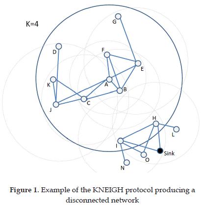
Two versions of this protocol were proposed in order to maintain only bidirectional links between nodes and their neighbors [14]. The main drawback of this protocol is the fact that it does not guarantee connectivity, due to the probabilistic fact of the selection of the parameter k. Figure 1 shows an example of a reduced topology using KNEIGH in which the selected k does not provide connectivity. The XTC protocol is a modified version of the KNEIGH which guarantees connectivity by exchanging neighbor tables among nodes in order to avoid eliminating links that will disconnect the network. This protocol presents two disadvantages: the message exchange will generate extra overhead, because each node will have to send a potentially long message to its neighbors; and, in addition, the complexity of the analysis of the tables and their size may be greater than the computational and memory capacity of the nodes, especially in very dense networks. The KNEIGH-Tree protocol addresses these problems of possible lack of connectivity, extra overhead and large 2-hops away neighborhood tables by adding a sequence to the execution of the protocol (which is usually random among the nodes in the network) and taking advantage of the tree structure to guarantee connectivity, while keeping a message complexity of 1 packet per node, and a list of just 1-hop neighbors. The simplicity of this protocol is the main reason why it has been selected for this test. This protocol will be explained with more detail in Section 3.

Apart from reducing the transmission power of the nodes, the second main way to implement topology construction is by reducing the number of active nodes in the network. This method is also divided in different subcategories: backbone-based, cluster-based and adaptive.

The first and second categories are the most commonly implemented in the literature, while the third is less common: all of them find a small set of nodes that perform the tasks of the network and send the rest of the nodes to a low-energy consumption mode, but they differentiate in the sense that the first defines a connected structure; the second one finds clusters of nodes that share dependence on a special node per cluster, which is in charge of communication and maybe other tasks; and finally the third one which defines whether or not the nodes are active based on performance metrics of the network (lost packets, coverage, density of active nodes, etc.). Some examples of algorithms of the second and third kind are in [16, 17].

Two examples of protocols of the first kind mentioned above, which create a communication backbone, are the A3 [18] and A3Cov protocols. These protocols find a Connected Dominating Set (CDS) on the graph and turn off all the nodes that do not belong to the CDS. These protocols guarantee connectivity among the nodes in the network and have a low message overhead, bounded by no more than 4 and 5 messages per node respectively. The A3 protocol has been tested among other CDS-based algorithms and has successfully produced smaller or similar sized trees with lower message complexity and energy usage. The A3Cov protocol has been compared with the coverage-oriented TCn protocols and it has been seen that, in dense networks, it provides coverage of at least 90% of the maximum network coverage. Both these protocols have shown good results in terms of lifetime and message complexity, which makes them good choices to represent the protocols of this kind. These protocols will be explained with more detail in Section 4.

The purpose here is to evaluate and compare the KNEIGH-Tree, a transmission power-based topology construction algorithm, against the CDS-based A3 and A3Cov protocols, in terms of their impact on the network's lifetime, in order to contribute with an answer to the question asked in the title of this work: is it more energy efficient to reduce the communication range of the nodes or turn them off as methods of extending the lifetime of the network?

The KNEIGH-Tree is a topology construction protocol that modifies the network topology by reducing the transmission power of the nodes depending not only on how many nodes they reach, as its predecessor the KNEIGH protocol presented in [14], but also taking into account which nodes are being reached; these characteristics guarantee at least 1-way connectivity along the network to the sink. The main contribution of this protocol is its use of the features of a tree structure in order to define a connected reduced topology. The KNEIGH-Tree follows a "growing a tree" technique: the process starts at a predefined node, usually the sink node, and progresses sequentially, level by level. Using this technique, instead of a purely random execution, provides a powerful tool to guarantee connectivity in the network: if every node can reach at least one other node in a lower level on the tree (hops from the initial node), then the network can guarantee that every node will have a path to the sink.

This is an extension to the original work in the sense that before, the protocol did not have any information about the network's topology in order to make such decisions, and depended only on probability of connection based on the parameter k. In some sense, the new approach may cause parameter k to lose some importance given that connectivity can be reached by the tree level condition; however, the tree level condition can only guarantee 1-way connectivity and parameter k is an auxiliary to bi-directionality. Based on this, KNEIGH-Tree can be executed in two modes: Tree level only, and K+Tree level. The first one will reduce the transmission range to reach only the closest lower-level node, while the second will try to cover the first k neighbors and also reach the closest lower-level node.

The KNEIGH-Tree protocol

The way the protocol is executed is as follows: Every node starts in an Unvisited state. The sink node sends a HELLO message to all its neighbors at maximum power, which includes its ID number and its tree level. The node that receives the HELLO message stores the sender's ID and tree level, calculates the distance with the sending node (based on the RSSI or another technique), and sets its state to Visited. After receiving the HELLO message for the first time, a node sends a HELLO message of its own to its own neighbors and sets a timer in order to listen for its neighbor's messages.

After the timer expires, each node sorts its neighbors list, which it created from the HELLO messages, in ascending order and starts selecting which nodes will be part of its final neighborhood. Depending on the execution mode, the node will select its neighbors in the following way:

1. Just tree level: find the closest neighbor with lower tree level.

2. Just K: select the first k neighbors (similar to the original KNEIGH)

3. K + Tree level: select at least the first k neighbors or until finding the closest neighbor with lower tree level.

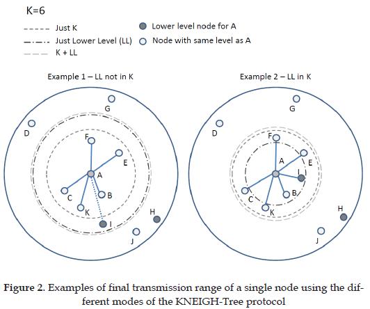
After finding the set of neighbors, each node sends an UPDATE message to announce its new neighborhood and then the nodes reduce their transmission ranges in order to reach only the farthest edge of their reduced neighborhoods. An example of the execution of the modes can be seen in Figure 2. In Section 5 the three execution modes will be compared in terms of coverage and lifetime.

The KNEIGH-Tree protocol assumes that the nodes have no knowledge of their positions, and that they can modify their transmission power in a continuous manner. Using a discrete number of power levels will be studied in a future work. The computational complexity of the protocol depends directly on the selected sorting algorithm, while the message complexity is of 2 messages per node, which could be reduced to 1 message if the UPDATE message is not sent.

The A3 and A3Cov protocols are topology construction protocols that, instead of reducing the transmission power of the nodes as the KNEIGH-Tree does, calculate a network backbone in order to guarantee connectivity and coverage, respectively, and then they turn off all redundant nodes in the network, so their energy is preserved for future maintenance, i.e. replacing the nodes whose energy is depleted with nodes whose energy was not used. The main idea behind these protocols is that the nodes may save more energy by going to a very low energy consumption mode, or sleep mode, while they are not needed, instead of just reducing the transmission power (which only saves energy when the nodes have to send a packet) and keeping the electronic components of the node active and consuming energy.

The A3 and A3Cov protocols work using the "grow a tree" technique to calculate the reduced topologies. A3 only creates a tree-like connected reduced topology that guarantees connectivity along the network, but does not concern itself with coverage. All the leaf nodes can be sent to sleep because they do not provide connectivity to any other node in the network. Given that the main objective of the WSNs is to monitor events, creating a backbone for connectivity may not be enough to guarantee coverage of events. For this reason, the A3Cov protocol creates a backbone that provides connectivity to the network, as does its predecessor, but it also selects extra nodes that extend the sensing coverage of the network compared to the original A3 protocol. This reduction offers several advantages to the network:

1. The energy in the sleeping nodes is not used until the node is needed, so the consumption due to idle operation is reduced.

2. By reducing the number of active nodes, the amount of messages that the network is transporting is also less.

3. Less nodes transmitting implies less competition for the channel, which may reduce latency and probability of collisions.

In general, all these facts have an impact on the rate of energy consumption of the network, which should extend the lifetime of the network.

The A3 protocol

The way the A3 protocol works is as follows:

1. All nodes start with the Unvisited state, except the stating node, which starts with the Active Candidate state.

2. An Active Candidate node sends a HELLO message to all its neighbors. The first one that sends this message is the sink node. In addition, this node sets a timer to wait for replies from Unvisited neighbor nodes.

3. All the neighbors send back a PARENT RECOGNITION message that includes their ID and their own selection metric, which is a convex combination of the ratio or remaining energy in the receiver, and the ratio of distance over the maximum transmission range. Also they adopt the sender as their "parent" nodes, and change their state to Child.

4. After a period of time, the Active Candidate node stops listening for messages, sorts the list of "children" nodes (neighbors who answered) in a decreasing order, and sends this sorted list back to its children. If the Active Candidate node has received at least one answer, it will change its state to Active; otherwise, it will change its state to Sleeping and will turn off its components until the next topology maintenance routine is executed.

5. The children nodes find themselves in the list and wait for a period of time proportional to their position on the list.

6. When the timer in a node expires, and it has not received any SLEEPING messages, the node will send a SLEEPING message, change its state to Active Candidate and go to step 1.

7. If the node receives a SLEEPING message while in the timer set in step 4, it will change its state to Sleeping Candidate, and will turn off its component for a period of time. After this timer expires, the node will change its state to Active Candidate and go to step 1.

This algorithm has been shown to allow every node in the network to finish as an Active or Sleeping node, and also to guarantee connectivity among the nodes in the network. In addition, it presents a low message complexity of O(n), bounded by 4n, where n is the number of nodes in the network. The computational complexity of A3 is O(n Log n) due to the sorting algorithms executed by every node. Figure 3 shows an example of the execution of the A3 protocol in a topology with 200 nodes, uniformly distributed along a square area of side 600m, with communication range of 100m and sensing range of 50m. A3 selected 40 out of 200 nodes to be active in order to preserve connectivity in the network, and a coverage ratio of 70.9%.

The A3Cov protocol

A3Cov works very similarly to A3, but presents important changes in some of its steps; for example, during step 3, if there are any nodes that have not received any PARENT RECOGNITION messages, it means that there are no nodes that depend on it for communication purposes; however, they may still be useful in order to extend the network's sensing coverage. In order to do this, A3Cov defines a new variable in the nodes called sensing covered: a node x is sensing covered by node y if x is inside the sensing range of y and y is an active node (d(x,y) < R_Sense). If a node is sensing covered it is assumed that its contribution to the total coverage of the deployment area is not enough to keep it active. If an Active Candidate node does not have any answers (at the end of step 3) it will go to step 7 (continued from step 6 of A3 above).

1. If the node has been sensing covered by any other node (including its parent node), it sets a short timer to wait for SENSING COVERED messages from its active neighbors.

2. If the timer expires and the node is not sensing covered yet, it will turn itself on, change its state to Active and send a SENSING COVERED message and a SLEEPING message. If any node in its range receives the SENSING COVERED message, it will evaluate if it has been covered by the sender, in which case it will update the value of the sensing covered variable.

3. If, during the timer set in step 7, the node received a SENSING COVERED message from any other node, it will stop the timer, change its state to Sleeping and turn its components off until the next topology maintenance routine.

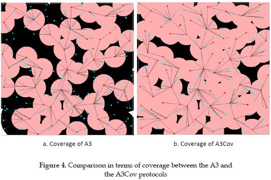
A3Cov expands considerably the coverage provided by the A3 protocol, but just adds a single message to the message complexity of O(n), now bounded by 5n, and makes no change in the computational complexity. Figure 4 shows a comparison in terms of coverage between the A3 and the A3Cov protocols when applied to the same topology defined in Figure 3a. A3Cov provides a coverage ratio of 91.44% of the area, using 66 active nodes. The ratio of coverage is 22.46% higher than the one provided by A3 alone, but the number of active nodes are also increased by 65%. These two variables show a tradeoff between the size of the active topology and the area of coverage, which appears to be non linear. This relation is out of the scope of this paper and will be studied in a future work.

In the next section, these two protocols are compared with the KNEIGH-Tree protocol in order to determine how these protocols really allow the network to preserve energy and extend its lifetime compared to the option of not having any topology construction scheme at all.

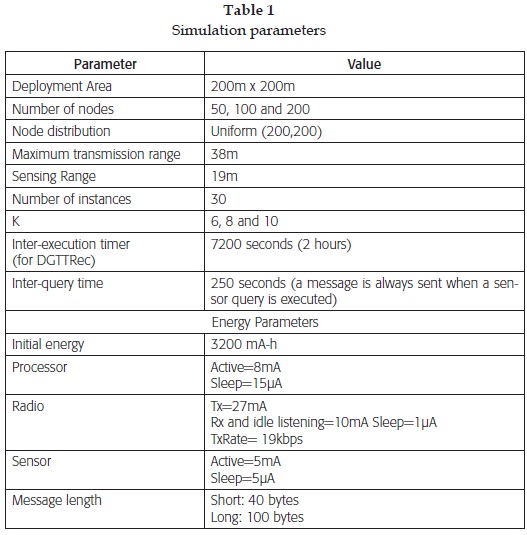
The evaluation of the protocols is performed in the following stages: first, the KNEIGH-Tree protocol is studied in order to characterize its behavior in terms of coverage in time, according to the network density and the parameter k. Based on these results, the best configuration is compared with the results from the A3 and A3Cov protocols, also in terms of coverage in time, in order to compare their level of extension of the network's lifetime. The detailed definition of the parameters for the scenarios can be seen in Table 1.

In order to guarantee that maximum use of resources in the network, a topology maintenance protocol is included in the experiment: the Dynamic Global Time-based Topology Recreation (DGTTRec) has been selected for this experiment due to its simplicity and that it periodically will update the network's topology based on the current state of the nodes. All the experiments in this section were performed in Atarraya, a simulation tool for topology control. This simulator is being offered under the GNU licensing agreement and the topologies could be requested for reproduction.

The metrics being measured in the experiments in this section are coverage and lifetime. Coverage here is defined as area covered by the sensing area of all active nodes reachable by the sink node; in other words, if an active node cannot reach the sink node, its coverage is not taken into account in the coverage metric. The definition of lifetime used here is based on declaring the networks death when the sink node has no active node in its neighborhood, in which case it is isolated and cannot receive information from the network.

The experiments in this section use three different scenarios: sparse, medium dense and dense networks. The sparse network is defined as the one that, given a set of nodes n, the initial communication radius used is defined as the Critical Transmission Range according to [20]. This guarantees that the node degree is very low and the network is weakly connected. The medium dense and dense scenarios use the same communication radius but increase the number of nodes by 2 and 4 times the original one, which augments the node degree and the connectivity in the network. Three values of k were considered (6, 8 and 10) in order to show the impact of this parameter.

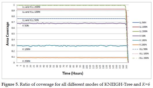
First, it can be clearly seen that, no matter the execution mode, the network barely lives above 168 hours. This behavior reflects that the greatest impact on the lifetime of the network is due to the fact that all nodes are active for the duration of the network, especially the ones close to the sink node. If a single node would stay active but idle, the initial battery charge would last 171 hours; thus the sensing and communication related activities only decrease the life of the network by three hours, equivalent to just 1.5% of the total energy used by the network to remain active.

The second conclusion is that the Just K mode of KNEIGH-Tree (or the original KNEIGH protocol) does not produce good coverage with the k parameter used here, especially when increasing the network size: with 50 nodes coverage is close to 70%, while with 100 and 200 nodes it is around 30% and 10%, respectively. This confirms the findings in [13] where they proved that with larger network size, a higher node degree was necessary to guarantee connectivity, and thus, connectivity. In order to confirm that larger k would help to increase coverage, Figure 6 shows the results of comparing coverage when using parameter k with values 6, 8, and 10. In order to get more details about the last hours of the network, so that the best configuration could be defined, Figure 6 only includes results from the 162nd hour of activity, from which the coverage starts to decline.

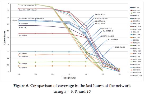
As it can be seen from the results, incrementing the value of the parameter k affects positively the level of coverage of the KNEIGH-Tree in Just K mode, reaching the maximum potential coverage of the network for 50 nodes (76% of area coverage) and increasing coverage from 8% to 14% and 24% for 200 nodes, and from 23% to 56% and 73% for 100 nodes, with parameter k 6, 8 and 10, respectively. Based on the experiments results, these ratios of coverage are still very low compared to the solutions provided by the Just Lower Level and K+Lower Level of the KNEIGH-Tree protocol. These two modes provide equal level of coverage due to the inclusion of the LL restriction in the selection of the transmission range of the nodes, because this feature guarantees connectivity in the network, thus the coverage provided by all the active nodes in the network can be used. In order to guarantee a higher level of coverage for the Just K mode it would be necessary to apply the formula in [13] and define the best value for k, for the given scenario. This could become a trial-and-error procedure which would create overhead in the network or could end up selecting a value for k so high that it would generate the MaxPower graph, showing no savings in energy.

The difference between the LL and the KLL modes can be seen in the way the coverage decays during the last hours. In all three different network sizes and for all values of parameter k, the LL mode preserves higher coverage than the KLL mode, in some moments having up to 17% more coverage. This advantage can be explained by the savings in terms of energy by not having to increase the transmission range to reach more neighbors than the one needed for connectivity (the one with lower tree level). In general, the impact of increasing the parameter k in the KLL mode is the reduction of the actual coverage in the last hours of network's activity.

The conclusion of this first experiment is that the Lower Level mode provides the best lifetime among all the KNEIGH-Tree protocol's modes and it will be used in the comparison with the A3 and A3Cov protocols in the following section. The parameter k has no impact on the LL mode, thus it is not necessary to define for the next experiment.

Experiment 2 - Comparison of KNEIGH-Tree LL, A3, and A3Cov

This section compares the coverage and network's lifetime provided by the three topology construction protocols KNEIGH-Tree, A3, and A3Cov.

As shown in Figure 7, in general, the network lifetime using the A3 and A3Cov protocol always goes beyond the 168th hour threshold that was unattainable by KNEIGH-Tree; however, the KNEIGH-Tree always provides higher coverage during that first part of the network's active time.

In the scenario with network size N=50, A3 and A3Cov provide a covered area of 52% and 69%, while KNEIGH-Tree covers 76%. The lifetime extension provided by the A3-based protocols is not very relevant in terms of coverage, given that providing just 20% or less coverage is not useful for any real application that needs adequate sensing coverage. In this case, the KNEIGH-Tree may be preferred due to the higher coverage ratio. The low extra contribution of the A3-based protocols is due to the low network density: the number of neighbors of the sink is very low, so they are needed all the time in order to provide connectivity, so their energy usage is very similar to the nodes in the KNEIGH-Tree protocol.

In the next scenarios with larger network sizes, the extension in lifetime and coverage increases considerably. Even though there is still some reduction at the 168th hour, this can be defeated by replacing the depleted sink neighbors with the extra ones that were sent to sleep. For example, with N=100 nodes, KNEIGH-Tree starts covering 92% of the area and A3Cov and A3 just 84% and 59%, respectively, but A3Cov can provide up to 50% area coverage for another 130 hours after the KNEIGH-Tree threshold; furthermore, when N=200, KNEIGH-Tree starts by covering 99% of the area while A3Cov and A3 only cover 93% and 67%, respectively, but A3Cov can provide coverage of over 80% for 230 more hours and 50% over 420 hours, and A3 can provide coverage over 50% after more than 600 hours past the threshold of 168 hours.

Increasing the network size has a positive impact on the behavior of the A3-based protocols because the number of active nodes that they need in order to provide connectivity or coverage does not grow linearly with the network size. On the contrary, they eventually find a stable value, no matter how large the network grew. Thus, the amount of sleeping nodes grows with the network size, and all those nodes become tools to extend the network's lifetime when they can replace the depleted nodes.

This article gives an initial answer to the question about which topology construction strategy produces better results, those that reduce the transmission power of the nodes or those that turn nodes off. Three different protocols are presented and compared in terms of coverage and network lifetime: the KNEIGH-Tree protocol, which reduces the transmission power of the nodes while guaranteeing connectivity, and the A3 and A3Cov protocols, which calculate a CDS tree and turn unnecessary (redundant) nodes off.

The results showed that in sparse networks, the KNEIGH-Tree is a good option because it provides the maximum coverage that the network can offer, and the extension provided by the A3 and A3Cov is too small to provide any advantage in real applications. However, despite the size of the network, KNEIGH-Tree showed a lifetime threshold of 168 hours of continuous activity before the network was unusable due to the synchronized depletion of the sink's neighbors and the consequent isolation of the sink node from the rest of the network.

On the other hand, with dense networks, the A3 and A3Cov protocols take advantage of the rising amount of redundant nodes using their energy resources for maintenance purposes, extending the network's lifetime; however, this means that the network will need more nodes in order to guarantee redundancy. For example, in the scenarios with 200 nodes, A3Cov could preserve over 80% area coverage for 230 hours after the 168 hours that the network using KNEIGH-Tree lasted. A topic to be studied in the future would be how the network's lifetime would behave if instead of having large initial networks, periodical redeployments were performed after the activity thresholds, like the one that KNEIGH-Tree showed.

[I] P. Santi, Topology Control in Wireless Ad Hoc and Sensor Networks. England: John Wiley and Sons, 2005.        [ Links ]

[2] M. Labrador and P. Wightman, Topology Control in Wireless Sensor Networks. New York, NY: Springer Science + Business Media B.V., 2009.         [ Links ]

[3] K.R. Gabriel and R.R. Sokal, "A New Statistical Approach to Geographic Variation Analysis," Systematic Zoology, vol. 18, pp. 259-270, 1969.         [ Links ]

[4] G. Toussaint, "The Relative Neighborhood Graph of a Finite Planar Set," Pattern Recognition, vol. 12, pp. 261-268, 1980.         [ Links ]

[5] B. Delaunay, "Sur la sphère vide," Izvestia Akademii Nauk SSSR, Otdelenie Matematicheskikh i Estestvennykh Nauk, vol. Vol. 7, pp. 793-800, 1934.         [ Links ]

[6] V. Rodoplu and T. H. Meng, "Minimum Energy Mobile Wireless Networks," IEEE Journal of Selected Areas in Communications, vol. 17, no. 8, pp. 1333-1344, 1999.        [ Links ]

[7] N. Li, J.C. Hou and L. Sha, "Design and Analysis of an MST-based Topology Control Algorithm," presented at IEEE Conference on Computer Communications, 2003, pp. 1702-1712.        [ Links ]

[8] A.C. Yao, "On Constructing Minimum Spanning Trees in K-Dimensional Spaces and Related Problems," Journal in Computing of the Society for Industrial and Applied Mathematics, vol. 11, no. 4, pp. 721-736, 1982.        [ Links ]

[9] L. Li, J.Y. Halpern, P. Bahl, Y.M. Wang and R. Wattenhofer, "A Cone-Based Distributed Topology-Control Algorithm for Wireless Multi-Hop Networks," IEEE/ACM Transactions on Networking, vol. 13, no. 1, pp. 147-159, 2005.        [ Links ]

[10] L. Kleinrock and J. A. Silvester, "Optimum Transmission Radii for Packet Radio Networks or Why Six is a Magic Number," presented at IEEE National Telecommunication Conference, 1978, pp. 4.3.1-4.3.5.        [ Links ]

[II] J. Ni and S. Chandler, "Connectivity Properties of a Random Radio Network", IEE Proceedings Communications, vol. 141, no. 4, pp. 289-296, 1994.        [ Links ]

[12] T. Hou and V. Li, "Transmission Range Control in Multihop Packet Radio Networks," IEEE Transactions on Communications, vol. 34, no. 1, pp. 38-44, 1986.        [ Links ]

[13] F. Xue and P.R. Kumar, "The Number of Neighbors Needed for Connectivity of Wireless Networks", Wireless Networks, vol. 10, no. 2, pp. 169-181, 2004.        [ Links ]

[14] D.M. Blough, M. Leoncini, G. Resta and P. Santi, "The K-Neigh Protocol for Symmetric Topology Control in Ad Hoc Networks", presented at 4th ACM International Symposium on Mobile Ad Hoc Networking and Computing, 2003, pp. 141-152.        [ Links ]

[15] R. Wattenhofer and A. Zollinger, "XTC: A Practical Topology Control Algorithm for Ad-Hoc Networks", presented at 18th International Parallel and Distributed Processing Symposium, 2004.        [ Links ]

[16] W. Heinzelman, A. Chandrakasan, and H. Balakrishnan, "Energy-Efficient Communication Protocol for Wireless Microsensor Networks", presented at 33rd International Conference on System Sciences (HICSS), 2000, pp. 1-10.        [ Links ]

[17] A. Cerpa and D. Estrin, "Ascent: Adaptive self-configuring sensor networks topologies", IEEE Transactions on Mobile Computing, vol. 3, no. 3, pp. 272-285, 2004.        [ Links ]

[18] P. Wightman and M. Labrador, "A3: A topology control algorithm for wireless sensor networks", presented at IEEE Globecom, 2008.        [ Links ]

[19] P. Wightman and M. Labrador, "Atarraya: A simulation tool to teach and research topology control algorithms for wireless sensor networks", presented at 2nd International ICST Conference on Simulation Tools and Techniques, March 2009.        [ Links ]

[20] M. Penrose, "The Longest Edge of a Random Minimal Spanning Tree", The Annals of Applied Probability, vol. 7, no. 2, pp. 340-361, 1997.        [ Links ]