


 English (pdf)
 Article in xml format
 Article references
 Send this article by e-mail
 Cited by SciELO
  Cited by Google
  Similars in
SciELO
Similars in
SciELO  Similars in Google
 Permalink
INTRODUCTION
Climate and atmospheric scenarios have been approached by a variety of researchers to acquire knowledge of interest. Environmental, climatic, and meteorological information has been used to determine behaviors and patterns within the studied area [1]-[12], and air pollutants have been used to understand the formation and impact of natural disasters and greenhouse effect within a region [13]-[16], be it to predict situations, relate causes and effects, and take measurements of the area to finally provide improvements, conclusions, and considerations in favor of the environment.
Currently, many algorithms are used to process records in the analysis of climate data, as shown in Table 1, which compiles more than 30 studies that used clustering algorithms for climate data, using various sources of information, records, timelines, and various objectives.
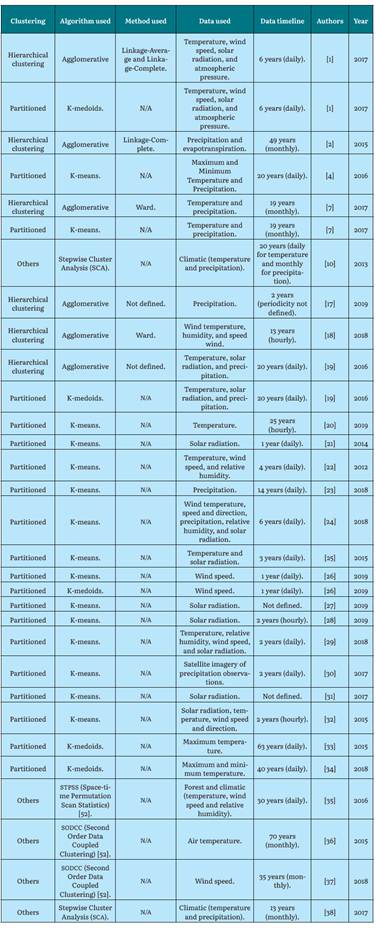
As shown in Table 1, K-means, K-medoids, and hierarchical grouping are the clustering algorithms most used by the authors.
Researchers approached various clustering algorithms (Agglomerative, K-means) [1], with various methods where they applied climate data with a series of metrics to find performance, especially computational performance. Other studies used clustering tools to observe the behavior of the data according to the number of established clusters [22]. Different works recommended some grouping models for specific environmental data by looking for the best projections of particulate matter in the studied region [24]. Also it was demonstrated the proper techniques to view annual temperature trends [34]. Other studies obtained, with proposed partitioned algorithms, the best precipitation estimates in the studied regions [30] and it was used clustering to improve noise reduction in analysis of solar radiation and temperature parameters [19]. Finally, other works used comparisons between unsupervised algorithms using climate data to find higher returns on them [32].
However, there is no clear guidance on which algorithm and parameters specifically serve to obtain the best results with the available data. Therefore, this research focused on working in that gray area to know and understand the behavior of some unsupervised machine learning algorithms applied to various scenarios with climate data.
In order to address this issue from experimentation, the guiding question of the paper is proposed as: How do clustering algorithms behave in different scenarios for climate data processing?
METHODOLOGY
The methodology includes the stages of variable selection, definition of the climatic seasons, obtaining the data set, definition of the scenarios, creation of the scenarios, and choice of tool for the execution of the algorithms. Then, it includes the results and its analysis.
Selection of Climatic Variables
To carry out the investigation, the following four meteorological variables were taken into account: temperature, precipitation, relative humidity, and solar radiation. These variables were selected for being the most reported in the state-of-the-art review in climate research with clustering algorithms [1], [2], [4], [7], [10], [20], [29], [31]-[33], [37]-[39].
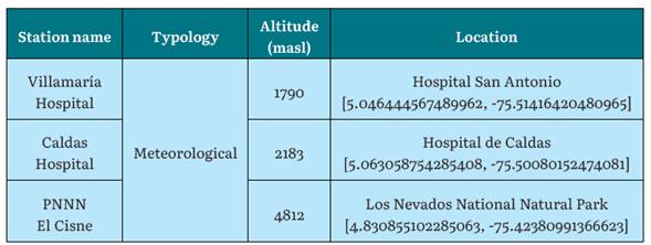
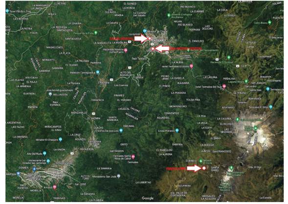
Definition of the Climatic Stations
Data from three meteorological stations called Villamaria Hospital, Caldas Hospital, and Los Nevados National Natural Park (El Cisne) were used, which comprised of 430.635, 530.802, and 248.297 instances, respectively. Table 2 shows the information of the stations.
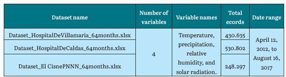
Obtaining the Data Set
To obtain the records, the data warehouse of the Caldas Environmental Data and Indicators Center (CDIAC) was accessed. The data warehouse is a climate records storage system for the entire department of Caldas, administered and managed by the Adaptive Intelligent Environment Group (GAIA). It is also a project lead by the IDEA (Environmental Studies Institute) of the National University of Colombia, Manizales branch. The data warehouse is a large storage structure implemented in PostgreSQL that houses more than 60 million environmental data, whose information is collected from more than 100 stations, including meteorological stations located in different geographic sectors throughout the department, and whose information can be viewed through http://cdiac.manizales.unal.edu.co. SQL queries were executed to extract the required data from the data warehouse to form the datasets. The records are between April 12, 2012, and August 16, 2017 (time range that contains the whole required data), comprising 64 months (5.3 years) with a data periodicity of every 5 minutes, and for this period information is extracted from the four climatic variables to be analyzed. Table 3 shows the retrieved datasets.
Definition of Scenarios
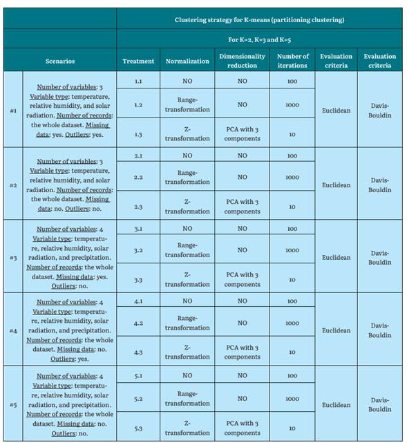
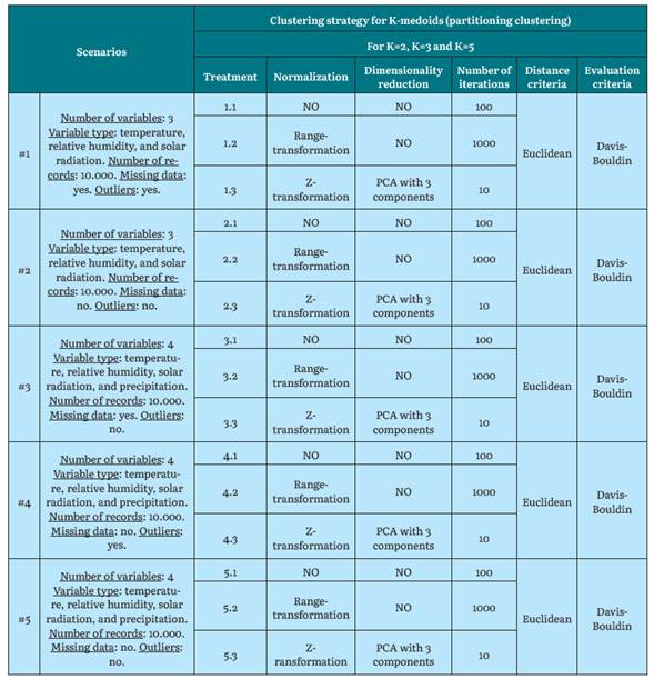
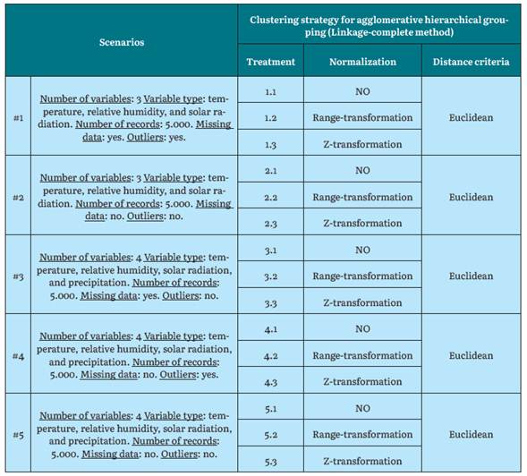
The scenarios are the defined environments where the clustering algorithms are applied, with a diversity of characteristics and parameters to, therefore, analyze and understand how the algorithms behaved in each of these scenarios. The parameters for each scenario are number of variables, type of variable, number of records, missing data, and presence of outliers, which, combined with the characteristics of each station, represent an interesting spectrum for the evaluation of the algorithms.
Different algorithms and modifications in some execution parameters are applied on the data related to the defined scenarios and on the selected stations.
Clustering algorithms: The three clustering algorithms most used by researchers in the analysis of climate data were selected. Agglomerative hierarchical grouping with Linkage-complete, K-means, and K-medoids for partitioned grouping.
Number of clusters (K): The generation of three different groupings whose K value were 2, 3, and 5 was proposed. This selection was based on results from other authors [1], this was corroborated by applying the elbow method in one of the cases, which validated these ranges.
Normalization: For experimentation, normalization with Z-transformation and range-transformation was used as part of the process of reducing value scales in the variables.
Dimensionality reduction: Principal Component Analysis (PCA) was used. The used variables were the four ones: relative humidity, temperature, precipitation, and solar radiation.
Number of algorithm iterations: For experimentation, iteration values of 1, 10, 100 and 1000 were used, where each value is ten times greater than the previous one.
Distance measurement: Euclidean distance was used as the distance function, considered to be the most reliable [1], and being used in a wide variety of jobs in the climate field [2], [7], [18], [19], [30], [33], [40], [41].
Cluster Quality Assessment: This metric consists of evaluating the result of the grouping to determine the quality of the clustering. For experimentation, the Da-vis-Bouldin index was used as a proposed metric for evaluating cluster quality [1], [22], [42H45].
Scenario Creation
Some work scenarios are defined for each one of the three algorithms. These scenarios are configurations to be taken into account in the executions to test each algorithm with different metrics.
Choice of Tool to Execute the Algorithms
To create the scenarios and run the algorithms, we chose to use Rapid Miner (version 9.2), a data mining software used for the analysis of a data set using a variety of operators, tools, and functionalities. It has been used by the scientific community in environmental issues [25], [46H49] given the versatility and options it allows, as well as the confidence it generates due to its proven effectiveness.
RESULTS
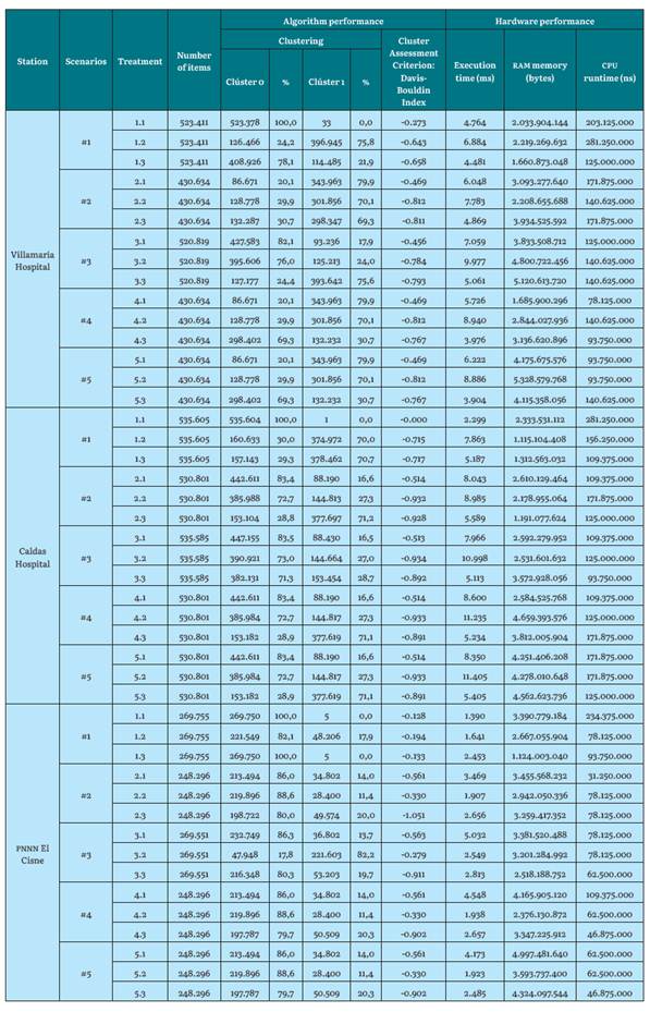
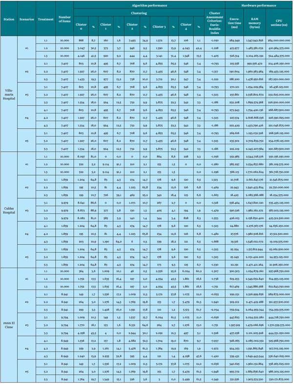
The results obtained from algorithm and hardware performance for K-means, K-medoids, and Hierarchical Grouping for each of the stations are presented in Tables 7, 8, 9, 10, 11, 12, and 13. Each one of the three weather stations of the region (Villamaría Hospital, Caldas Hospital, and Los Nevados National Natural Park) are K = 2, K = 3, and K = 5, respectively.
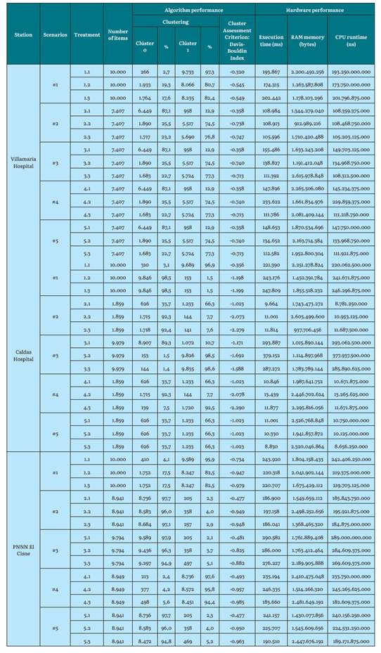
Table 7 Algorithm and hardware performance results for K-means with K=2 for the Villamaria Hospital, Caldas Hospital and PNNN El Cisne stations
Source: the Authors.
Table 8 Algorithm and hardware performance results for K-means with K = 3 for the Villamaria Hospital, Caldas Hospital, and PNNN El Cisne stations
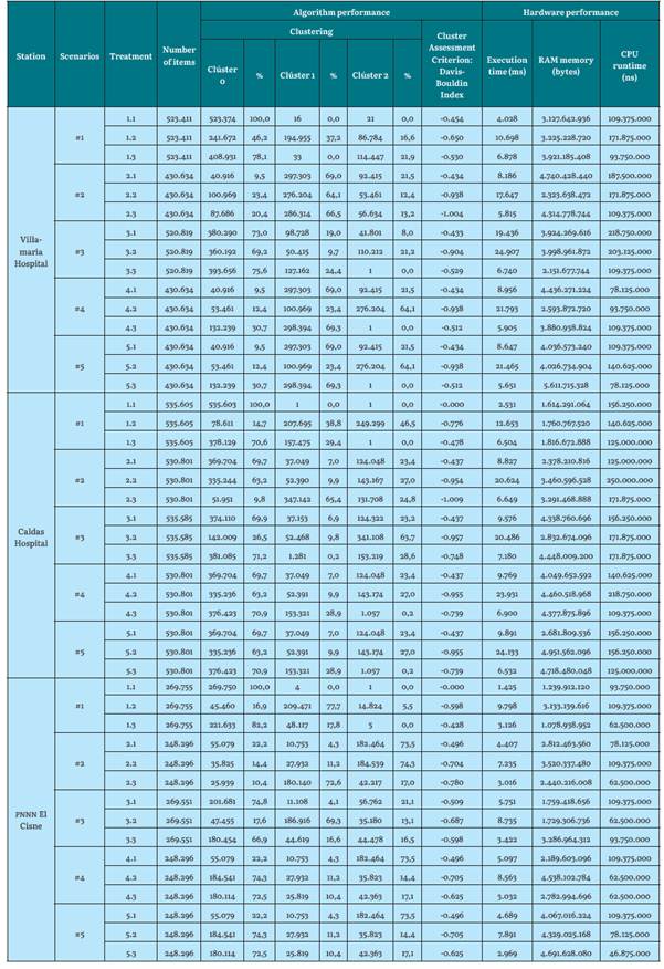
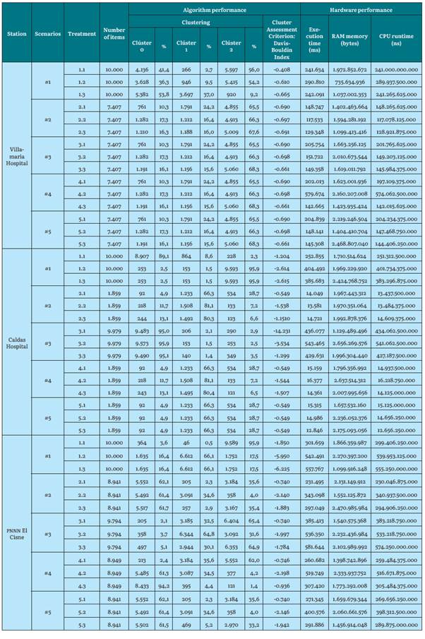
Table 9 Algorithm and hardware performance results for K-means with K = 5 for the YillamarIa Hospital, Caldas Hospital, and PNNN El Cisne stations
Source: the Authors, from previous work [39]
In a global view, for the Hospital de Villamaria station (low altitude), the evaluation indices for all its scenarios and treatments are observed. Regarding the Hospital de Caldas station (intermediate altitude), the evaluation indices are lower than the previous station (gaining quality), and they also remain similar for the rest of its K values. However, for the El Cisne PNNN station (maximum height), quite the opposite happens: The evaluation Davis-Bouldin indices (clustering lose quality) [1] and remain the same for their K values.
Regarding K-means, iterating the algorithm to form clusters by assigning each point to its closest centroid and recalculating the centroid of each cluster is a very efficient and simple process, not only by executing two steps for each iteration, but also by seeing how it is able to process immense quantities of instances very quickly. In its experimentation with the Hospital de Caldas station, it used more than 530.000 instances. This coincides with the contribution of [22], by defining K-means as a simple and efficient algorithm.
The execution times of the K-means algorithm increase as the value of "k" is greater. This is because you must iterate more times due to the need to create more clusters. For stations such as Hospital de Caldas and Villamaria, the execution times are higher since there are datasets of more than 430,000 instances. For the El Cisne PNN station, the execution times are shorter since they comprise a dataset of less than 250,000 instances.
ram memory consumption is very similar for all k values and for the three weather seasons. Although it differs in certain work scenarios, the average consumption is 2.6 Gb of ram. This means that regardless of the characteristics of the scenarios and datasets, ram uses, on average, the same amount of resources because its consumption is given the minimum it needs to run the algorithm's functionality.
The cpu runtime increases as the value of k increases. This is due to the processing it uses for the number of clusters to generate. The same behavior is observed for the three climatic stations.
Table 10 Algorithm and hardware performance results for K-medoids with K=2 for the Villamaria Hospital, Caldas Hospital, and PNNN El Cisne stations
Source: the Authors.
Table 11 Algorithm and hardware performance results for K-medoids with K = 3 for the Villamaria Hospital, Caldas Hospital, and PNNN El Cisne stations
Source: the Authors.
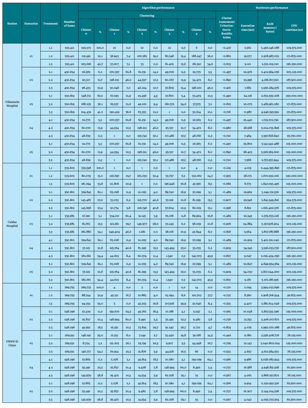
Table 12 Algorithm and hardware performance results for K-medoids with K = 5 for the Villamaria Hospital, Caldas Hospital, and PNNN El Cisne stations
Source: the Authors, from previous work [39]
Regarding K-medoids for the Hospital de Villamaria station (low altitude), the evaluation index becomes lower as the value of K (number of clusters) increases. For the Hospital de Caldas station (intermediate altitude), the evaluation indices are lower than the previous station and the greater the number of groups, the value of these indices is still lower (gaining quality). However, for the El Cisne PNNN station (maximum height), the opposite is true: the evaluation rates are, once again, higher (losing quality).
For previous partitioned algorithms (K-medoids, K-means), standardization and technique type greatly influence the evaluation of cluster quality. The Davis-Bouldin index, when evaluating the quality of the cluster, generates an approach (and visually verifies) the best grouping result. Furthermore, the higher the K value, the more hardware requirements and time requirements will be demanded to execute and process a dataset, and, subsequently, to execute the algorithm.
Also, note that K-means and K-medoids cannot process empty fields. Some authors omit missing and corrupt data from these algorithms [1], therefore the missing data was transformed to an average value of the attribute. This decision was supported by experts in the matter and made to allow the algorithm to run. Also, the average value corresponds to the whole dataset. We did not want to replace it with the lower or higher value because this would generate dragging of clusters, and it would alter the analysis of the results. The research shows a notable difference between clean datasets versus datasets with missing values that are replaced by an average value of the attribute, since, in the results, there is variation in the grouping evaluation index, which is better when the dataset is clean. On the other hand, the datasets with missing data and atypical data (scenario 1) produced the lowest performance results. This is due in part to there being an imbalance in the formation of the clusters and the evaluation index of their treatments not being the best. This signifies that using a raw dataset is not recommended. Furthermore, the outliers did not affect the results, since the clustering evaluation indices given by scenario 4 are very similar. For example, in scenario 5, which uses a clean dataset. This could be due to the fact that the outliers number was small compared to the dataset size (outliers subject to existence within the dataset), or, conversely, normalization allowed for reducing these large distance margins to provide better groupings.
It also corroborates the idea that applying dimensionality reduction with PCA, where three components are obtained, raises the level of abstraction of the results, since it does not allow for direct visualization of the map of the original attributes. As it was mentioned [42], that data transforming from an original space into a new one with a lower dimension, where they cannot be associated with the characteristics of the original, means that an analysis of the new space is very complicated and complex, since there is no physical meaning for the transformed and obtained characteristics.
Therefore, promoting a PCA with two components could determine the behavior of the data in a two-dimensional plane and make its analysis easier. In turn, this brings the reduction of initial attributes (which are four) to only two. In terms of clustering evaluation, PCA did not influence the improvement of the Davis-Bouldin index.
On the other hand, the number of iterations forces the algorithm to form the clusters and recalculate the centroids more times. However, it reaches a point where it finds the calculation it needs without improving with more iterations. As seen in experimentation, a number of iterations in 100 was a balanced value for working with clustering, where computational performance in terms of execution times is not affected for the algorithm. This prevents an investigator from unnecessarily repeating thousands of times. It is verified that iterating with a larger number does not affect the improvement of the evaluation index (recalculating its centroids to find a suitable value).
Table 13 Hardware performance results for Linkage-Complete for the YillamarIa Hospital, Caldas Hospital, and PNNN El Cisne stations
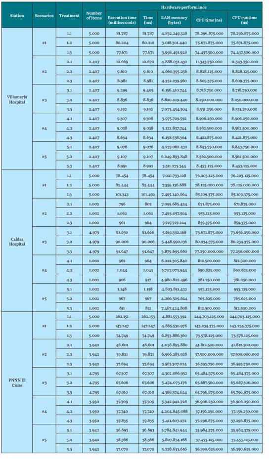
Source: the Authors.
For the agglomerative clustering algorithm, we decided to process with 20,000 instances to test the previous algorithm operation and determine the subsequent creation of the scenarios. The processing was found to be too slow. This was due in part to the algorithm presenting great computational complexity. Once a distance measurement is determined and used, a dissimilarity matrix is constructed. This process leads to the generation of a 20,000 x 20,000 size matrix (for a dataset of 20,000 instances), which, in hardware terms, requires storage and processing resources. After this, the data sets are merged at each level and the difference matrix is subsequently updated. This has a great impact on computer processing, and execution takes more than 1 hour and 30 minutes (for a dataset of 20,000 instances). That is, it took 72 times more than the previous 5,000 instance scenarios. This conclusion supports the research of [1], where hierarchical grouping is not recommended for a dataset of more than 10,000 instances. Therefore, it was decided to create scenarios with data sets not exceeding 5,000 instances.
Hierarchical grouping cannot process empty fields. With that said, the missing data was transformed to an average value of the attribute.
In terms of attributes, precipitation makes the dendrogram more complex to analyze, not only because it creates an additional agglomeration in the lower levels, but also because it involves increasing the dataset with thousands of more data. This leads to the graph agglomerate creating many instances, as well as becoming narrow for subsequent visualizations and analyzes. Due to the initial dataset being large, it is recommended to use precipitation for a dataset that guarantees a lower number of instances than those used in this experimentation; that is, below 1,000 instances for the agglomerative algorithm.
Based on the above data, a dendrogram of around 3,000 instances (sheets) can allow an investigator to easily see how the instances merge from the intermediate level, and focus the observation on higher levels, despite the lower levels being impossible. To visualize them, a researcher must evaluate from level 0 of the tree. It is suggested to use data sets of less than 100 instances for the dendrograms to be more visible, allowing better analysis from the lowest levels. Hierarchical grouping is preferred for a small dataset [1], [50].
On the other hand, normalization facilitated the construction of dendrograms, helping the dissimilarity and similarity distances (Y axis) to become closer on a scale between zero and one. This allowed the dendrogram to be viewed in a more simple manner. The dimensionality reduction was not transcendental in the results, therefore, it is concluded that it was not useful for the agglomerative algorithm.
In computational terms, the algorithm uses similar machine resources in all the scenarios, regardless of the preset characteristics. However, if high execution times and CPU times are found for scenario 1 (up to eight times greater than the rest of the scenarios, with only 2,000 instances apart), confirming that using datasets with large instance volumes for agglomerative hierarchical grouping can lead to slow processing.
DISCUSSION
To determine, in a preliminary study, the behavior of clustering algorithms on climate data, stations and datasets with different characteristics, scenarios were defined to which variants of the learning algorithms were applied, and the behavior of the metrics was evaluated.
The results, without being conclusive, can guide people who work with these data in the speedy selection of these elements, which we consider the contribution of this work.
For K-means, at the Hospital de Caldas station, there are more clustering evaluations with better quality compared to the other two stations. This is determined by taking a value as a reference to make the count. In this case, the indices are equal to or below -0.700. It could be given by the fact that a dataset whose attribute values do not contain extreme conditions (such as high or low temperatures), is associated to better clustering evaluation indices, with this algorithm.
For K-means, the best clustering evaluation index for the Hospital de Villamaria station had a value of -1,004, as opposed to the Hospital de Caldas station, which had a value of -1,009. These best results are given for the climate dataset extracted from a region that oscillates between 1790 msnm and 2183 msnm (between warm and temperate climates), using K-means with a value of K = 3, performing normalization with transformation Z and a number of 10 iterations.
Regarding the El Cisne pnnn station, a dataset that comes from high altitude sources, such as 4,812 meters above sea level, the best evaluation index was of -1,051, with a value of K = 2, normalization with Z-transformation, and a number of iterations of the algorithm in 10.
On the other hand, for K-medoids, at El Cisne PNNN station, there are more clustering evaluations with better quality compared to the other two stations. This is determined by taking a value as a reference to make the count. In this case, the indices equal to or below -0.700. It could be given by the fact that a dataset whose attribute values contain extreme conditions (high temperatures or relative humidity of the 100%), such as the El Cisne pnnn station, generate an approximation to better clustering evaluation indices for the clusters in K-medoids.
For K-medoids, the best clustering evaluation index for the Villamaria Hospital station had a value of -1,405, these best results are given for a climate dataset extracted from a region that oscillates around 1,790 masl (warm climate), when using K -medoids a value of K = 5 clusters, normalization with Z-transformation, and number of algorithm iterations in 10.
For the Hospital de Caldas station (altitude of 2,183 masl, temperate climate), the best index had a value of 14,231, using a value of K = 3, without any other characteristic. Regarding the El Cisne pnnn station (4,812 meters, extremely cold weather), the best clustering evaluation had a value of -7,937 and used a value of K = 5, without any other characteristics.
Based on the above and the information seen in the Results section, the cluster evaluation indices are observed with very low values for K-medoids, compared to those obtained in K-means. For two partitioned algorithms used in the experimental framework, the algorithm that presented the best performances and results was K-medoids.
For Linkage-Complete agglomerative clustering, dataset processing that contains the fewest instances and has gone through a normalization process with Range-Transformation performs best on dendrograms, in graphic terms. Even though having fewer instances makes the dendrogram easier to visualize and analyze, normalization makes it possible to shorten similarity distances (Y axis). A performance evaluation index or performance cannot be applied to this algorithm because it is hierarchical clustering and researchers must develop external functionalities in software to provide performance evaluations at a mathematical level [51], and to determine at what point they want to cut the tree to obtain a value of clusters (K), and, from there, analyze the results.
The contribution sought with this work is to provide some basic guidelines, so as not to start from scratch, on certain decisions in the analysis of clusters with meteorological data, as well as to help identify the algorithm and the most important parameters to take into account for the best performance, in accordance with the particular conditions and requirements [52].
CONCLUSIONS AND FUTURE WORK
For future work, it is recommended to use other types of scenarios, treatments, algorithms, and other amounts of clusters to see performance evaluations. It would also be important to know how to evaluate hierarchical agglomerative algorithms to determine the quality of dendrograms to break the subjectivity of each researcher and to apply mathematical measurements.
Furthermore, carrying out scenarios with a K value greater than 5 would allow researchers to investigate what happens with clustering and performance for partitioned algorithms (K-medoids, K-means), both at the machine level and in their performance.
On the other hand, evaluating data on a time scale (per day, per week, etc.) using time series would allow for knowing interesting clustering behaviors, as well as the quality of their clusters within a timeline for different seasons, or times of the year (how the performance would be given for cold seasons or summer seasons). Also, it would be interesting to perform processing under different scenarios that comprise a larger data set (of millions of instances) for K-means, in order to better observe the computational behavior on a larger scale. This will help determine how efficient it is for large datasets, to better detect new patterns or relationships.
Based on the results, it is possible to suggest using other normalization methods, such as ratio and interquartile range transformation, to see how clustering behaves with these analyzes.
It is recommended to use techniques, such as Ordinary Kriging, to handle the large amounts of zeros that a variable contains within a dataset.

