USE OF NEURAL NETWORKS IN PROCESS ENGINEERING
Thermodynamics, diffusion, and process control and simulation applications

ABSTRACTT

This article presents the current status of the use of Artificial Neural Networks (ANNs) in process engineering applications where common mathematical methods do not completely represent the behavior shown by experimental observations, results, and plant operating data. Three examples of the use of ANNs in typical process engineering applications such as prediction of activity in solvent-polymer binary systems, prediction of a surfactant self-diffusion coefficient of micellar systems, and process control and simulation are shown. These examples are important for polymerization applications, enhanced-oil recovery, and automatic process control.

Keywords: process engineering, neural networks, process control, process modeling, process simulation.

RESUMEN

El presente artículo presenta el estado actual de la utilización de las Redes Neuronales Artificiales (ANNs) en aplicaciones de ingeniería de procesos donde los métodos matemáticos tradicionales no muestran completamente el comportamiento representado por observaciones y resultados experimentales o datos de operación de plantas. Este artículo muestra tres ejemplos de la utilización de ANNs en aplicaciones típicas de ingeniería de proceso como son la predicción de coeficientes de actividad en sistemas binarios solvente-polímero, predicción de coeficientes de difusión de un surfactante en sistemas micelares y control y simulación de procesos. Estas aplicaciones son importantes en el área de polimerización, recuperación mejorada de crudo y control automático de procesos.

Palabras clave: ingeniería de procesos, redes neuronales, control de procesos, modelado de procesos, simulación de procesos.

INTRODUTION

Neural network definition and theory

Artificial neural networks (ANNs) is a type of artificial intelligence, and an information processing technique, that attempts to imitate the way human brain works. It is composed of a large number of highly interconnected processing elements, called neurons, working in unison to solve specific problems. The organization and weights of the connections determine the output. The neural network is configured for a specific application, such as data classification or pattern recognition, through a learning process called training. Learning involves adjustments to the connections between the neurons. Neural networks can differ on: the way their neurons are connected; the specific kinds of computations their neurons do; the way they transmit patterns of activity throughout the network; and the way they learn including their learning rate (Haykin, 1994).

ANNs have been applied to an increasing number of real-world problems of considerable complexity. Their most important advantage is in solving problems that are too complex for conventional technologies; problems that do not have an algorithmic solution or for which and algorithmic solution is too complex to be found. The ANNs are able to learn and to generalize from a few specific examples and are capable of recognizing patterns and signal characteristics in the presence of noise. ANNs are inherently nonlinear and, therefore, capable of modeling nonlinear systems (Bhat, and McAvoy, 1990; Savkovic-Stevanovic, 1994; Basheer, 1996).

Topology of a neural network

The topology of a neural network is the logic structure in which multiple neurons, or nodes, are intercommunicated with each other through synapses that interconnect them. The synapses (biological term) are the interconnections between nerve cells in biological networks and have been sometimes extended to ANNs.

Figure 1 presents a schematic diagram of a typical neural network. The circles represent the processing neurons and the interconnection lines are the information flow channels between neurons. The boxes are neurons that simply store inputs to the net. Each processing neuron has a small amount of memory and executes a computation which converts inputs to the neuron into outputs. The computation is called the transfer function of the neuron. The transfer function can be linear and nonlinear and consists of algebraic or differential equations. The network shown in the figure has three layers of neurons: input, hidden, and output.

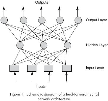
Figure 2 shows the structure of a single neuron within an arbitrary network. The inputs to this neuron consist of an N-dimensional vector P and a bias, B_j, whose value is 1 multiplied by a weight. Each of the inputs has a weight W_ij associated with it. Biases give the network more degrees of freedom which are used to learn a desired funtion.

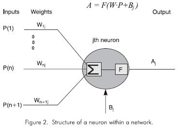
The first calculation within the neuron consists in calculating the weighted sum of the inputs plus the bias:

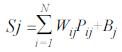
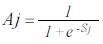
The output of the neuron is afterwards calculated as the transfer function of S_j. This transfer function can be a step-change, a linear, or a sigmoid transfer function. The linear transfer function calculates the neuron's output by simply returning the value transferred to it. The sigmoid transfer function generates outputs between 0 and 1 as the neuron's net input goes from negative to positive infinity. The sigma function is described as:

Once the outputs of the hidden layer are calculated, they are transferred to the output layer.

Neural Network Training

Once a network architecture has been selected, the network has to be taught how to assimilate the behavior of a given data set. Learning corresponds to an adjustment of the values of the weights and biases of every single neuron interconnection so a satisfactory match is found for input-output data. There are several learning rules, such as nonlinear optimization and back- propagation, but the common aim is to minimize the error between the predicted value, obtained by the network, and the actual value. Three training methods were used in this paper: backpropagation, Levenberg- Marquardt (LM) minimization, and Random Activation Weight Net (RAWN). A brief description of each method follows but for greater detail the reader is referred to references (Rumelhart, 1986; Hagan and Menhaj, 1994; Te Braake, 1997).

A backpropagation network learns by making changes in its weights and biases so as to minimize the sum of squared error of the network. The error is defined as the subtraction of the actual and predicted value. This is done by continuously changing the values of the weights and biases in the direction of the steepest descent with respect to error. This is called the gradient descent procedure. Changes in each weight and bias are proportional to that element's effect on the sum- squared error of the network.

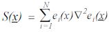
The LM minimization method is a modification of the classic Gauss-Newton method for nonlinear least squares. A detailed description of the methods can be found in Fletcher (1987) and in Hagan and Menhaj (1994). Both methods use an estimate of the Hessian, H=∇²V(x) (matrix of the second derivatives of the function to optimize with respect to the parameter vector x), and the gradient ∇V(x), where V(x)is the function to optimize, the sum of squared errors. x is the matrix of the weights of the corresponding network to train, and e(x)is the error matrix. An algebraic procedure makes it possible to express both the Hessian and the gradient in terms of the Jacobian matrix (Hagan and Menhaj, 1994). It can be shown that:

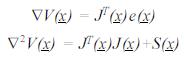
where the Jacobian matrix, J(x), is

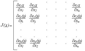
and

Gauss-Newton method assumes that S(x) ≈ 0. The update for the weights becomes:

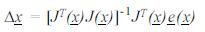
This equation is the one used in any Gauss-Newton optimization method. Levenberg-Marquardt (LM) modification is done by including the LM parameter μ, such that:

I is the identity matrix. The LM parameter is multiplied by some β factor whenever a step would result in an increased V(x). When a step reduces V(x), μ is divided by β. Notice that when m is small, the algorithm becomes the Gauss-Newton. Also notice that when m is large, the algorithm becomes steepest descent with a step of 1/μ. Let's remember that the approximate steepest (gradient) descent algorithm is described by:

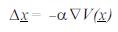
where α is the learning constant. If Δx is the matrix of changes in weights and biases, ΔW, the LM equation will become:

The software used in this work was MATLAB from Mathworks, along with its toolboxes of neural networks, optimization, and simulink. MATLAB performs a numerical calculation of the Jacobian.The LM algorithm is a simple modification to the backpropagation method. The implementations of this LM algorithm (or the Newton types) require intermediate storage of n·n matrices, compared to only a n element vector for the other backpropagation methods. When n is very large (such as for neural networks), this can become an issue and the latter algorithm may be preferred. LM training method is faster than backpropagation when the number of hidden layers is not high (i.e., higher than 15).

The RAWN method uses the fact that a three layer feedforward network, with neurons using the sigmoid function in one hidden layer, is theoretically capable of approximating any continuous function. If the weights between input and hidden-layer neurons are known, an estimation problem, that is linear in parameters, remains can be easily solved by standard least-squares methods. This learning method is very fast and the results are good. However, neither the number of neurons required in the hidden layer is known, nor whether a single layer is best for learning speed.

A well trained network tends to give reasonable values when presented to inputs that it has never seen. Typically, a new input will present an output similar to the correct output for input vectors used in training that are similar to the new input being presented. This property enables to train a network on a representative set of input/output-target pairs and obtain good results for new inputs without training the network for all the possible input/output pairs.

ACTIVITY PREDICTION WITH NEURAL NETWORKS (Polymer/Solvent binaries)

Artificial neural networks were used to predict activity of solvents in polymer solutions. The polymer- solvent systems considered were polar, nonpolar, and polar/nonpolar binaries. The data specifically used were the same ones used by Ramesh and his coworkers, who used another type of artificial neural network with a different learning rule, nonlinear optimization training routine (Ramesh, 1995).

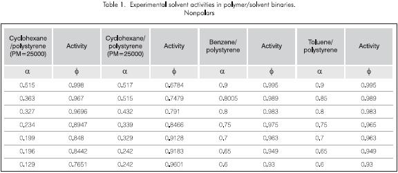
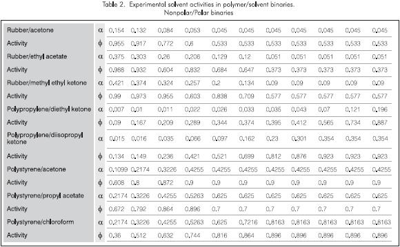
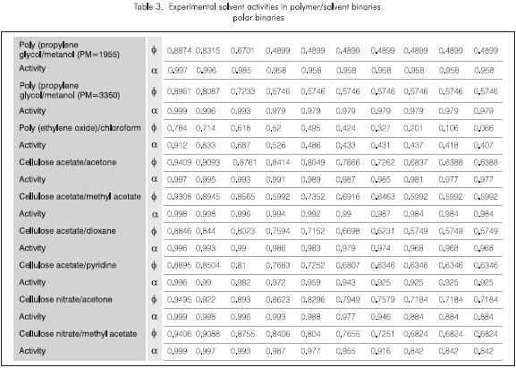
Tables 1, 2 and 3 show the experimental data used for the systems to be tested. They include four nonpolar binaries, eight nonpolar/polar binaries, and nine polar binaries. The experimental data used were obtained from Alessandro (1987) and include the binary type, the volume fraction of the polymer, Φ, and the solvent's activiy,α.

The neural network used for activity prediction

Figure 3 shows the network used for the solvent activity function approximation of our binaries. P is the matrix (RxQ) that represents the inputs for each binary system. The waffle of Q input vectors at the left of Figure 3 is used to represent the simultaneous presentation of Q vectors to a two layer sigmoid/linear network. Q represents the number of input vectors. That is, the number of data sets for each binary system. S1 is the number of neurons in the hidden layer. S1=10 was used for the three cases. S2 is the number of neurons in the linear output layer.

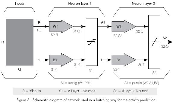
W1 and W2 are the matrices that correspond to the values of weights in the hidden layer (Layer 1) and the output layer (Layer 2), respectively. As well as with the matrices B1 and B2, which correspond to the bias matrices. These vectors could be serially presented to the network in order to train it. However, Q input vectors can be presented by simultaneously specifying the matrix P.

The architecture shown in Figure 3 is capable of approximating a function with a finite number of discontinuities with arbitrary accuracy. The layer architecture used for the function approximation of the solvent activity prediction in this project has a hidden layer of sigmoidal neurons (in this case tangent-sigmoid neurons). These neurons receive inputs directly and then broad- cast their outputs to a layer of linear neurons which computes the network output. The software package used to program this neural network was the Neural Networks Toolbox of MATLAB.

Results

Several networks were created and tested. The previous section described the parameters of the networks that showed the best results. The learning method used in all training sessions was the Levenberg-Marquardt method which was the one that gave the fastest training sessions, and adaptive backpropagation with momentum. A network for each polymer-solvent system was created. All the three created networks have a hidden sigmoidal layer and a linear output layer. Several numbers of neurons in the hidden layer were tried. The sum of squared error criteria for each binary type was 5·10^-4. The results of the predicted against the experimental values are very satisfactory for both training and testing sessions, according to the figures shown below. Figures 4, 5, and 6 correspond to the solvent activities obtained by the neural network model.

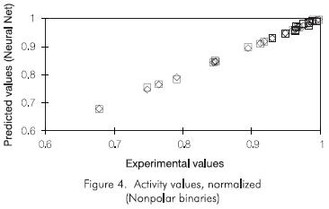
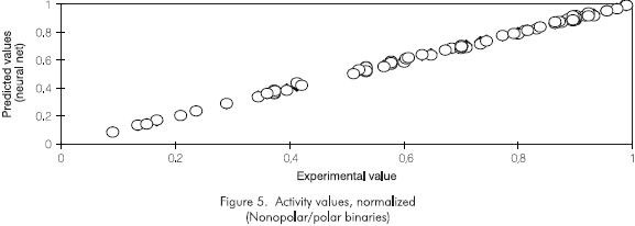
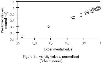
Figure 4 shows the predicted and experimental values for the nonpolar binaries. The training process took 4 epochs (iterations) to meet the error criteria using LM training method. The training session for the same system but using adaptive backpropagation took 1,600 epochs. There is a significant difference in the training time. All the points in Figure 4 fall on the 45 degree line indicating a very good agreement.

In the case of nonpolar/polar binaries, shown in Figure 5, the agreement is also very good. The training session with LM method took 8 epochs (iterations). The training with adaptive backpropagation did not reach the error criteria of 5·10^-4. After 15,000 a sum of squared errors of 4.5·10^-3 was reached with the backpropagation method.

Figure 6 below shows the results of the third type of binaries, the polar binaries, with a LM training session. The sum of squared error goal was the usual 5·10^-4. The results are quite acceptable. The same training session with backpropagation training reached a SSE of 1.5·10^-3 after 15,000 epochs. A large difference in the training times was also present.

These results are very similar to those obtained by Ramesh (1995) in his work on the same binaries. The proposed neural networks used in this work are also similar to those used by Ramesh. The difference lies in the application of the Levenberg-Marquardt training method that provides shorter training times.

DIFFUSION COEFFICIENT PREDICTION System: Micelles of sodium dodecyl sulfate

This section will initially explain the sodium dodecyl sulfate (SDS) micellar system. A description of the neural network designed to predict the self diffusion coefficient of SDS over a wide range of operating parameters such as temperature, concentration of SDS, and concentration of Sodium Chloride (NaCl), will be presented afterwards.

Micelles

Micelles are microheterogeneous assemblies. Examples of micelles are microemulsions that have been used extensively as media to carry out chemical reactions, to enhance solubilization of insoluble materials, to transport molecules through cell membranes, and also to treat waste water. These applications take advantage of the surfactant property of forming association complexes. The self-assembled surfactant micelles are dynamic fluctuating entities constantly forming and dissociating on a time scale ranging from microseconds to milliseconds (Fendler, 1982).

Surfactants, commonly called detergents, are amphiphatic molecules having distinct hydrophobic and hydrophilic regions. Depending on the chemical structure of their polar headgroups, surfactants can be neutral, cationic, anionic, or zwitterionic. The surfactant subject of this work is sodium dodecyl sulfate (SDS), an anionic surfactant.

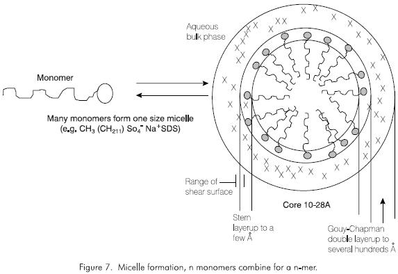
Over a narrow range of concentrations there is a sudden transition in the physical properties of aqueous surfactants. This transition corresponds to the formation of aggregates and is used to define the critical micelle concentration or CMC. This is an example of aggregating solutes in which solutes aggregate much more than the simple weak electrolytes. In the case of the detergent SDS, its molecules remain separate at low concentrations, but then suddenly aggregate. The resulting aggregates, called micelles, are most commonly visualized as an ionic hydrophilic skin surrounding an oily hydrophobic core (Figure 7). This is the way detergents clean; they capture oil-bearing particles in their cores.

SDS was chosen for this work due to several reasons. Among a variety of micellar systems, the one consisting of sodium dodecyl sulfate is the most extensively and systematically studied. The experimental properties of SDS micelles, such as diffusion coefficient, micellar radii, and aggregation behavior, have been well documented at various NaCl concentrations and over a wide range of temperatures.

The classical micelle is pictured as a roughly spherical aggregate containing 50 - 200 monomers. The radius of the sphere approximately corresponds to the extened length of the hydrocarbon chain of the surfactant. The micelle has a hydrocarbon core and a polar surface; it resembles an oil drop with a polar coat. The head- groups and associated counterions are found in the compact layer (Stern layer), as described by Fendler. Some of the counterions are bound within the shear surface, but the mayority are located in the Gouy-Chapman electrical double layer where they are dissociated from the micelle and are free to exchange with ions distributed in the bulk aqueous phase. The amount of free counterions in bulk water, expressed as a fractional charge, typically varies between 0.1 - 0.4.

Micelle diffusion coefficient estimation with neural networks

The diffusion coefficient (D) of micelles at various SDS and NaCl concentrations and over a wide range of temperatures (T) were taken from the literature and collected by Brajesh. 76 sets of data were used to train a feedforward neural network with a backpropagation learning algorithm 25 sets of data were used to test the net. The training set of data is shown in Table 4. Since sigmoidal forms of activation functions were used in the network, the network inputs and outputs were normalized so as to lie between zero and one. SDS concentrations (in molar units, M) and temperature (in °C) were normalized by dividing by 0.16 and 100, respectively. D, in m²s^-1, was normalized by dividing by 50·10^-11. NaCl concentrations (in molar units, M) were not normalized since they are all well distributed between 0 and 1 (Brajesh, 1995).

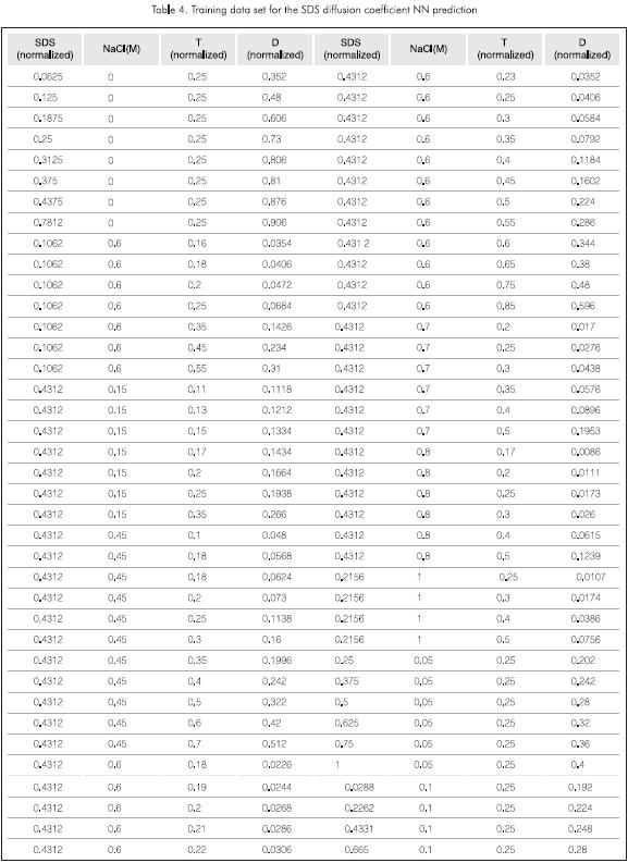
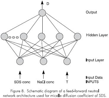
Figure 8 shows the network built to predict the self diffusion coefficient. The inputs for the network training were SDS and NaCl concentrations and temperature (both normalized). The output was the diffusion coefficient. The network architecture consists of three distributing neurons in the input layer, 10 sigmoid neurons in the hidden layer, and one linear neuron in the output layer.

Results

Figure 9 shows the real experimental data and the network-trained data. There is a good agreement. The model shows a good performance after training with both LM and backpropagation methods. However, LM training method needed 285 epochs (iterations) to reach the goal set for the sum of squared errors, SSE = 5.0·10^-4. Backpropagation with adaptive learning rate and momentum took 200,000 epochs to get an error of 1.0·10^-2.

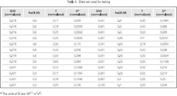
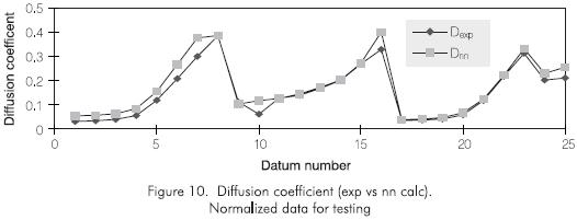
The trained network was given a new set of input data for testing. Table 5 shows the data presented to the network for testing. Figure 10 shows a plot of the predicted and experimental data for the diffusion coefficient of a micellar system of Sodium Dodecyl Sulfate. The network captures the behavior of the self diffusion with respect to SDS concentration, NaCl concentration, and temperature.

SIMULATION AND CONTROL OF A MIXING TANK

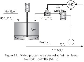
A final example of the applications of ANNs is the process control field. A mixing process, shown in Figure 11, will be simulated and controlled as an example by using a neural network based controller.

The training data were taken from the first principle model and simulation used by Camacho (1996) keeping assumptions and steady state values. The approach to control this process is the model based process control (MBPC) using neural networks. In this approach, a neural network process model is developed and used in a predictive basis. The neural network process model can be built by training a network with input-output data. Usually, a random signal with a zero order hold proportional to the process time constant is used to excite the manipulated variable. Another alternative way to excite the manipulated variable is with sinusoidal wave functions with frequency and amplitude chosen based on knowledge of process dynamics. The data produced in the manipulated and controlled variable are used to train the network.

Figure 12 shows the structure of the Neural Network Model Based Predictive Control (NNMPC). The NNMPC algorithm consists of minimizing an objective function which can be written in the general form:

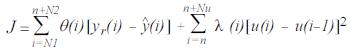
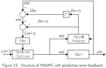
where α(i), the control signal to be sent out, is theunknown variable that will optimize J. y_r is the reference signal, or set point, is the model predicted output, θ is the set of prediction weighting factors that weight each prediction. N1 and N2 define the prediction horizon or the block of time in the future over which the error will be considered. N1- N2 is the length of this prediction horizon. λ is the set of control weighting factors, and its purpose is to prevent the controller from making large jumps. Nu is the control horizon, which normally is set to one time step due to extensive computation time when multiple υ values are used in optimization. N1 is usually n, the current time interval, although there have been some suggestions to take N1 as the process dead time (Cherré, 1998).

The neural predictor is the process model based on a neural network structure. The neural network model predicts the current value of the controlled variable when a set of inputs is given. The set of inputs often corresponds to the current and past values of the manipulated variable and past values of the controlled variable. When feedforward control scheme is desired, current and past values of disturbances may also be fed as inputs. The number of past values to feed as inputs to the neural network process model depends on the characteristics of the process, i.e., its steady state and dynamic behavior. Process parameters such as time constant and dead time define the number of inputs.

To alleviate steady state offsets due to small modeling errors, the difference between the actual plant output at time n and the ANNs prediction at time n is fed back to the optimizer. This prediction error is calculated at each time step and assumed constant over the entire prediction horizon. To account for model inaccuracies the error is added to all future predictions of y made in that time step. This would be represented as:

where _c (n+i) is the neural network prediction at time n+i corrected for the prediction error at time n.

Notice from Figure 12 that the error signal sent to the optimizer is first filtered in order to reduce the interference of noise and help with disturbance rejection. This introduces robustness and stability to the system. The filter suggested is a linear, first order one with a unity gain. y_r(t+1) is the reference signal or set point at time t+1 (García et al., 1988).

Neural network process model training

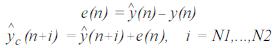
The training of the networks was performed using a random signal adequately covering operating region, shown in Figure 13. A zero order hold of five times the process time constant was placed on the signal. The zero order hold simply holds the random signal at its previous value for a prescribed amount of time. According to literature, and since the process time constant is based on a first order plus dead time, it can be said that the actual process will approximately reach steady state after five time constants have elapsed. (Smith and Corripio, 1997). The training method used was the regulated activation weight neural network (RAWN) which provides outstanding, short periods of training. It does not need iterations and requires a random activation and linear squares technique to train. The speed of computation is incomparably much faster than with backpropagation (Te Braake et al., 1997).

Testing the Neural Network Process Model

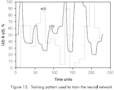
After training, the neural network process model is tested using more process data. Usually, two thirds of the data are used for training and one third is used for testing. The best source for training and testing data is past historical records of process behavior. The testing is also evaluated by checking the sum of squares of the model prediction errors on the training data set. Other criteria used are the sum of squares of the errors of the one step ahead predictions on the testing data, the sum of squares of the errors of the free run predictions on the testing data, and the sum of squares of the errors or the corrected free run predictions on the testing data. Figure 14 shows the testing results produced with a neural network of 15 neurons in the hidden layer. This network architecture produced the best criteria for the network evaluation. The figure shows a very good match from a free run test.

Neural Network Predictive Control

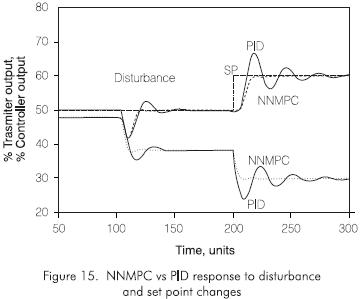
The NNMPC strategy shown in Figure 12 was implemented using MATLAB computer software along with its Neural Network Toolbox, Optimization Toolbox, and Simulink simulation package. A step change in disturbance W₁, the hot stream flow rate, from 1.89 kg·s^-1 to 1.51 kg·s-1 lb/min, was performed at time t = 100 times units, while the set point was constant at a value of 50% transmitter output. Then a step change in set point, from 50 to 60% transmitter output, was performed at time t = 200 times units. For comparison purposes, the same step changes in disturbance and set point were performed with a Proportional-Integral-Derivative (PID) controller tuned for this process. Results are shown in Figure 15.

Results

For this specific example, the performance of the neural network model predictive controller is better than that of the traditional PID. This is true for both disturbance and set point changes; at least in the range worked in this application. Further studies should explore the response of each controller to several disturbance(s) and set point changes. An evaluation of the integral of the absolute error of the controlled variable from the set point (IAE) and the integral of the absolute move in the manipulated variable (IAM) will provide another criteria for performance evaluation. Robustness and adaptability are also to be evaluated (Cherré, 1998).

GENERAL CONCLUSIONS

• ANNs are capable of handling complex and nonlinear problems, can process information very rapidly, and are capable of reducing the computational efforts required in developing highly computation intensive models for finding functional forms for empirical models.

• In ANNs, only input and output data are needed for the network to recognize the pattern involved in mapping the input variables to the output response. It is true that a neural network has been described as a "black box" solution for a problem. But the ability of ANNs to give rapid and accurate values in the case of process engineers makes ANNs a very useful tool. Their ability to easily perform the inverse problem, that is interchanging the input and the output vectors of the net, also makes ANNs appealing. This kind of analysis is very helpful in diagnostic analysis of an existing system.

• Whenever experimental data or historical plant data are available for validation, neural networks can be put to effective use. The application of neural networks as a predictive and diagnostic tool for the process engineering is therefore very promising and more investigation is being done

• ANNs can be efficiently used to simulate and control processes. In the specific example shown here, the performance was better than that of the traditional PID controller. There are also examples of ANNs use in multivariable process control. As well as examples of automatic control systems installed in refineries and petrochemical industries. ANNs constitute another resource for developing process control strategies in highly nonlinear processes that can show some trouble when controlled by more traditional methods. (Martin, 1997; Thompson, 1996).

• The following are other conclusions more relative to the specific neural networks created in this work:

• Correlations for evaluating activities in polymer- solvent systems and diffusion coefficients of an SDS micellar system have been obtained by using artificial neural networks.
• The networks evaluated polymer-activity and diffusion coefficients in good agreement with the experimental observations.
• Process simulation and control is another field in which ANNs can be used. In complex, nonlinear processes, they can offer an efficient performance when other traditional control techniques do not meet stability and performance requirements.

REFERENCES

Alessandro, V., 1987. "A simple modification of the Flory- Huggins theory for polymers in non-polar or slightly polar solvents", Fluid Phase Equilib, 34: 21 - 35.        [ Links ]

Basheer, A. I. and Najjar, Y. M., 1996. "Predicting Dynamic Response of Adsorption Columns with Neural Nets", Journal of Computing in Civil Engineering, 10 (1): 31- 39.        [ Links ]

Bhat, N. and McAvoy, T. J., 1990. "Use of Neural Nets for Dynamic Modeling and Control of Chemical Process Systems", Computers Chem. Engng., 14 (4/5): 573 - 583.        [ Links ]

Brajesh, K. J., Tambe, S. S. and Kulkarni, B. D., 1995. "Estimating Diffusion Coefficients of a Micellar System Using an Artificial Neural Network", J. Colloid & Interface Science, 170: 392 - 398.        [ Links ]

Camacho, O., 1996. "A New Approach to Design and Tune Sliding Mode Controllers for Chemical Processes", Ph.D. Dissertation, University of South Florida, Tampa.        [ Links ]

Cherré, D., 1998. "Use of Artificial Neural Networks in Process Control", Master of Science Thesis, University of South Florida, Tampa.        [ Links ]

Fendler, J. H. and Fendler, E. J., 1982. Membrane and Mimetic Chemistry, Wiley- Interscience, New York.        [ Links ]

Fletcher, R., 1987. Practical Methods of Optimization, J. Wiley,        [ Links ]

García, C. E., Pretti, D. M. and Morari, M., 1988. "Model Predictive Control: Theory and Practice a Survey", IFAC Workshop on Model Based Control, June.        [ Links ]

Hagan, M.T. and Menhaj, M., 1994. "Training Feedforward Networks with the Marquadt Algorithm", IEEE Transactions on Neural Networks, 5 (6): 989 - 993.        [ Links ]

Haykin, S., 1994. Neural Networks. A Comprehensive Foundation, Macmillan College Publishing Company, N.Y.        [ Links ]

Martin, G., 1997. "Nonlinear Model Predictive Control with Integrated Steady State Model-Based Optimization", AICHE 1997 Spring National Meeting.        [ Links ]

Ramesh, K., Tock, R. W. and Narayan, R. S., 1995. "Prediction of solvent Activity in Polymer Systems with Neural Networks", Ind. Eng. Chem. Res., 34: 3974 - 3980.        [ Links ]

Rumelhart, D. E. and McClelland, J. L., 1986. "Parallel Distributed Processing: Explorations in the Microestructure of Cognition", MIT Press, Cambridge, MA, and London, England.        [ Links ]

Savkovic-Stevanovic, J., 1994. "Neural Networks for Process Analysis and Optimization: Modeling and Applications", Computers Chem. Engng., 18 (11/12): 1149 - 1155.        [ Links ]

Smith, C. A., and Corripio, A., 1997. Principles and Practice of Automatic Process Control, John Wiley & Sons, Inc., N. Y.        [ Links ]

Te Braake, H. A. B., Van Can, H. J. L., Van Straten, G. and Verbruggen, H. B., 1997. "Two-step Approach in Training of Regulated Activation Weight Networks (RAWN)", Engng. Applic. Artif. Intell., 10 (2): 157-170.        [ Links ]

Thompson, W., 1996. "How Neural Network Modeling Methods Complement Those of Physical Modeling", NPRA Computer Conference.        [ Links ]