


Services on Demand
Journal
Article
 English (pdf)
 Article in xml format
 Article references
 Send this article by e-mail
Indicators
-
 Cited by SciELO
 -
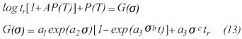
 Access statistics
Related links
-
 Cited by Google
 -
 Similars in
SciELO
Similars in
SciELO -
 Similars in Google
Share

 Permalink
CT&F - Ciencia, Tecnología y Futuro
Print version ISSN 0122-5383On-line version ISSN 2382-4581
C.T.F Cienc. Tecnol. Futuro vol.2 no.1 Bucaramanga Jan./Dec. 2000
ABSTRACT
An analysis was conducted on the creep behavior of HK.40 steel. This steel is high heat resistant, aged during service, under the conditions of a petrochemical furnace. The different models that describe its creep behavior are discussed. The tests were carried out under a constant load intending to simulate the operating conditions of a catalytic reforming furnace. Among the models proposed in the literature, the models of Degui, Jaske-Simonen, Larson-Miller, Manson-Haferd and Snedden were applied. Another model is proposed to account for the three stages of creep. The samples of the material have had from 74 to 88 thousand hours of service and are tested at a constant load until rupturing.
Key words: creep, tensile stress, deformation.
RESUMEN
Se efectuó un análisis del comportamiento en termofluencia del acero HK.40, resistente a altas temperaturas, envejecido en servicio, a las condiciones de un horno de petroquímica. Se discuten los distintos modelos que describen su comportamiento en termofluencia. Las pruebas fueron realizadas a carga constante tratando de simular las condiciones de operación de un horno de reforma catalítica. Entre los modelos propuestos por la literatura, se aplicaron el de Degui, Jaske-Simonen, Larson-Miller, Manson-Haferd y Snedden. Se propone otro modelo para explicar las tres etapas del fenómeno de la termofluencia. Las muestras del material tiene entre 74 y 88 mil horas de servicio y se ensayan a carga constante, hasta rotura.
Palabras clave: termofluencia, resistencia a la tracción, deformación.
INTRODUCTION
The main objective of this study was to determine the model that could predict the behavior of the material under creep conditions and during its service life. Having this model represents clear advantages for predictive maintenance systems, since it is possible to carry out changes in the equipment within a planned and reliable process. A Cr-Ni type steel alloy was chosen, classified as UNS J94224, corresponding to ASTM A608 HK-40 grade. The specimens selected for the experimental phase have had 74 thousand and 88 thousand hours of service in reforming furnaces belonging to the Barrancabermeja Refinery, having consumed over 50% of its design life. The damages due to creep in this type of furnaces are about 70% of the total causes of damage; while compared to another type (pyrolysis for instance) are about 30%. This is why the material mentioned was chosen for use in these furnaces.
Constant load equipment is used in the experimental methodology, simulating the efforts to which the material is service and aged is submitted in order to obtain the variations that occur in the constitutive models developed for new materials. This will improve the perception of the future behavior of the material in service or for the rest of its design life. At the material resistance laboratory of the Instituto Colombiano del Petroleo (ICP), the experiments have been conducted adding up to over 16 thousand hours, with systematic data compilation, reading time versus linear displacement.
THEORETICAL SETTING
Creep damage can be defined as the physical discontinuities observed in the grains, phases or grain boundaries in material structures operating at high temperatures.
Materials in general can behave (explained by the changes, sliding and/or dislocations that take place in the crystals or their granular structure); they can have plastic deformations (the structural changes are assumed as soon as they occur); or a viscous deformation (there is a delay in the deformation and they vary in time). A dislocation movement, a viscous deformation and a process of mass transfer (diffusion) occur simultaneously in creep. The latter can be explained in accordance wit the models of Cobe and Nabarro-Hering reported by Courtney (1990).
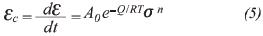
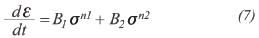
The basic variables of the creep theory are: stress ( ), deformation ( ), variation of stress in time (d /dt), variation of deformation in time (d /dt), and time (t). Also, the material properties depend on the temperature (T). Therefore, in a uniaxial state of deformations, the constitutive equations for materials submitted to creep have a general form:

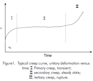
An assay of uniaxial stress is considered maintaining the stress or the load (since it is known that in a uniaxial test, the stress will change in proportion with the creep), and by determining the creep at each step in time, a curve of unitary creep can be obtained in function of Figure 1. Immediately following the application of the load, an elastic or plastic-elastic deformation occurs, indicated as, ε0. From there on, the load is kept constant and due to the temperature (constant throughout the assay), and the phenomena within the material, deformation increases. This is the viscous part, indicated as εv. This phenomenon is known as creep, where three stages can be distinguished: (I) a decrease in deformation rate (primary creep). The rate decreases continuously with time and the deformation, in most materials, forms a dislocation at the structure level of subgrains with a cell size that decreases as deformation increases. (II) At this stage there is a constant transient deformation (steady state or secondary creep). The microstructure is invariant indicating that recovery effects are occurring with the deformation at a constant deformation rate (steady state or secondary creep); and (III) at this stage, there is an increase in the transient deformation that precedes rupture (tertiary creep).
The formation, growth and spreading of the separation of grain boundaries are the main reason for degradation of mechanical properties, and specifically for a severe loss in the ductility of metallic materials.
Constitutive equations
Throughout the years, several researchers have tried to create and develop some type of formulation to entirely or partially explain creep. The difficulty that there is no unified mathematical law lies in the great quantity of variables that should be taken into account for each case. The diversity goes to the extent that it can be affirmed that practically every material can have its own unique mathematical rule and in each material, there can also be differences depending on factors such as: microstructure, quantity and quality of metallic and nonmetallic inclusions, thermal treatments, specific operating conditions, etc.
Most constitutive equations have been developed empirically for pure materials or assuming that they do not have type of internal damage. The most important ones historically are:
Where, εo: initial deformation; εc: creep; r: exponent depending on the temperature; t: time; εt : primary creep; dε/dt: steady state secondary creep.
The equation (2) formulated by Garofalo (Garofalo, 1965), for limited primary and secondary creep for materials working at temperatures between 0.05 and 0.3 of melting temperature, Tm. Today it is considered that a material is being submitted to creep when its operating temperature exceeds 0.4 Tm. This model does not mention the third stage of rupture, but it is important being that it covers the basic principles of the creep phenomenon.
Where, Q: activation energy [kJ/mol]; R: gas constant = 8.32kJ/kg-mol K; A0: constant. All other nomenclature is taken as mentioned in the paragraphs above.
Equation (3) is Arrhenius' law, applicable for the second stage or steady state creep. Figure 2 illustrates the tendency of this law.

Where, n: independent exponent of stress; B: constant. All other nomenclature is taken as mentioned in the paragraphs above.
Equation (4) F. H. Norton's proposal (Garofalo, 1965) and refers to the second stage of creep.
General equation for the uniaxial state
The general equation for the uniaxial state is made up of an elastic term and another one for creep (Creep in Metals, 1997). The term associated with the latter is a function of the three important parameters that rule (stress, temperature, activation energy), leading to a general equation for creep depending on stress and temperature in the form of:
which is a combination of the Arrhenius (3) and Norton (4) equations. The nomenclature is as mentioned in the paragraphs above.
Equation proposed specifically for HK-40 steel
For the particular case of the HK-40 material- object of this study - a constitutive equation has been proposed in the following terms, (Jaske and Simonen, 1991):
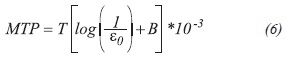
where, MTP: the model of primary creep, T: absolute temperature, B: a constant of the material, which for this case is 2.0, ε0 is the deformation from creep at the end of the first stage.
Jaske and Simonen (1991), recommend a ratio to determine the minimum deformation rate (or deformation of steady creep) as follows:
n is an independent stress exponent, the other nomenclature is taken as defined above.
Models to determine rupture time
There is a great variability of models (Vamas materials databanks, 1997) developed for design purposes to determine or extrapolate the rupture time of materials. Only some of them will be described here, for being considered the most important ones:
Larson-Miller Model, MLM
From equation (5), steady state creep F.R. Larson and J. Miller in 1952, developed a concept based on time-temperature joined as: T(K+log t) (Vamas materials databanks, 1997). It says basically that for a given material, the stress is illustrated against the MLM model. Once this value is obtained, the rupture time of the equation previously indicated can be found. This model is widely accepted and has been included in the API 530 standard of 1996. Taking equation (5) again, the MLM is developed as follows:

Where: C2: creep constant for the steady state (second stage); εII: secondary creep; tr: rupture time.
This equation is valid for constant stress. Taking the logarithm on both sides of the equality we get:

by regrouping, this comes to:

This is the Larson-Miller Model, is taken to a Log tr versus 1/T chart. A family of curves, at different stresses, coincide at one point on the axis of the ordinates (log tr), finding the value of the constant C (Larson-Miller constant) Figure 2.
Nevertheless, this model has the inconvenience of the calculation of constant C, which depends exclusively on the conditions of the material, but in the literature, there is a great variety of values for the same materials. On the other hand, MLM sets up a wide range of possibilities for rupture time, varying from a few hours to thousands of hours.
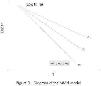
Manson-Haferd Model, MMH
This model developed by S.S. Manson and A. M. Haferd in 1953 (Vamas, 1997), is based on the same equation (5) but handles the concept of log tr versus T and arrives at:

A family of curves at different stresses coincide at the point that determines the values of Ta and log ta. Figure 3 illustrates this model.
The Degui Model
In 1990 (Vamas,1997) J. Degui proposed the following model to determine rupture time:

a,b: constants of the Degui model. All other nomenclature is taken as defined in previous paragraphs.
It is a simple model representing a linear relation between stress and time, the constants introduce the variable for temperature. The model is valid for stresses 200 MPa and should be found for each temperature.
MCM Rupture Model (Minimum Condition Method)
This model (Manson and Ensign, 1971 and Viswanathan, 1989) was developed to avoid the inherent danger upon selecting a particular model for a specific material. Up to now it is, according to the authors, the best model to adjust the data obtained due to its general expression, which allows the deduction of the other models. It has the following form:
This method proposed by S.S. Manson and C.R. Ensign in 1971, is considered the one for the future for approximations to rupture time. The difficulty in the application of this model lies in finding constants (ai,b,c) by experimentation and functions (G,P) numerically, which is to be carried out for the material in this investigation.
Snedden Model, 1977 (Vamas, 1997)
This is the simplest model to find rupture time in function of applied stress and for a specific temperature.
EXPERIMENTAL PROCEDURE
Characterization of the material
Samples are taken of the UNS J94224 type 25Cr-20Ni alloy, equivalent to an ASTM A-608 Gr. HK-40 from an H-1151 reforming furnace tube of the refinery with 74 thousand hours of service at an operating temperature of 1113K (840 °C) and a pressure of 3 MPa, and an H-4100 pyrolysis furnace tube with 88 thousand hours of service at 446 kPa and 1233K (960 °C). The material is an auste-nitic matrix steel casting with a mass presence of carbides. Melting temperature, Tm, 1503K (1230 °C), ultimate tensile stress (UTS) of 515 MPa, elastic stress of 345 MPa and a 17% elongation rate (6% for the aged material).
Methodology
For the laboratory experimentation phase, we have the material (described above); two sets of testing equipment at constant load and temperature. The load is applied on one set of equipment, by means of a multiplier. Over 16 thousand experimental hours were conducted, at different temperatures and deformations, continuously monitoring the values of deformation in time. The tests were programmed until the specimen ruptured. The data obtained are illustrated for each sample. They are analyzed and the generic behavior that can be used to trace a model is determined.
Results and Analysis
Figure 4 shows a photograph from an optic microscope where the cavities in the intergranular area are clearly observed in one of the samples tested. The sample is observed (tested at 1248K (975 °C) and 27 MPa) after the third stage, once the test tube has reached the rupture time of approximately 150 hours. The cavities have an average size from 8.4 m to 14 m. The aligned cavities are generated toward the grain boundary, as expected according to the Diffusion models of Nabarro- Herring and Cobe (Courtney, 1990) for temperatures greater than 0.4Tm. The results of the creep test are re. corded in Table 1 (Latorre, 1998). It was conducted on 36 samples, and the values corresponding to rupture time, final deformation and the value of minimum creep are registered.
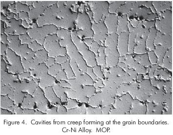
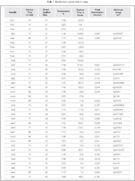
Figure 5 shows the tendency of the results according to the Manson-Haferd Model, MMH, chart calculated based on the data in Table 1 (Latorre, 1998). The data shows a tendency to obtain parallel lines contrary to what is supposed according to theory Figure 3, which however, allows the supposition of the values for Ta and log ta required to apply the MMH, according to equation 11. As can be observed, the curves tend to a non-convergence, which disqualifies this model, at least with regard to the material of this research.
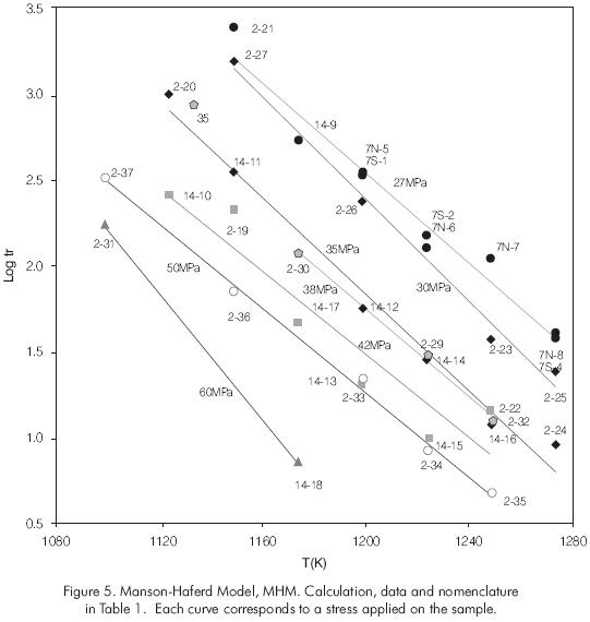
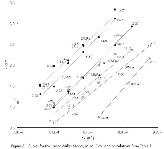
Figure 6 shows the tendency of the Larson-Miller Model, MLM, with a constant C (equation 10) of 15. In the chart, the value of the constant is indicated with the symbol (‡). It can be observed that the curves show a tendency to move away from this value, except for line 27 MPa, which would be right at the value of C if it were extended toward 1315K (1042 °C). This may be due to the fact that it is a low average stress and very close to the actual stresses in the pyrolysis furnace tubing. This almost parallel tendency coincides with what is observed by LeMay (1991) in his research on an austenitic material, which led them to redefine a model to adjust better than the MLM.
Figures 7, 8, 9, 10 (Latorre and Correa, 1998) show the differences between the MLM and the experimental data, in function of the load applied. An increasing differentiation is observed as the stress applied grows, but at the same time, it decreases with the increase in temperature. The values that predict the MLM (minimum) (API RP-530, 1996) have been included in Table 1.
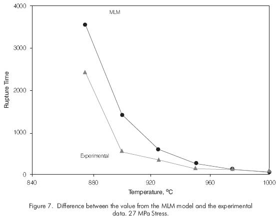
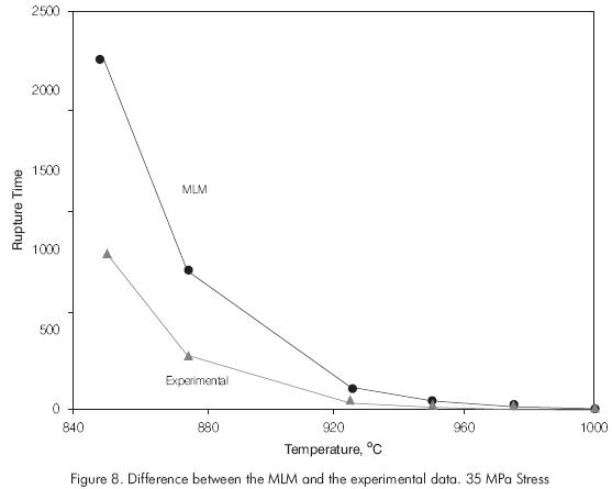
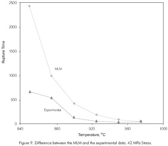
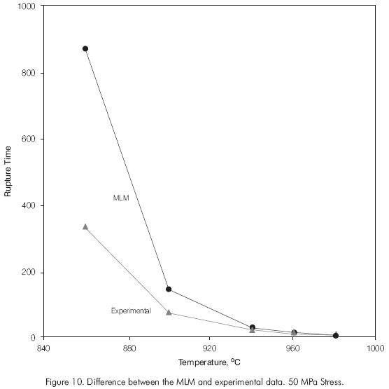
This model in general has a difference between 40 and 50% regarding rupture time found in the laboratory, which makes it very conservative for predictive maintenance work.
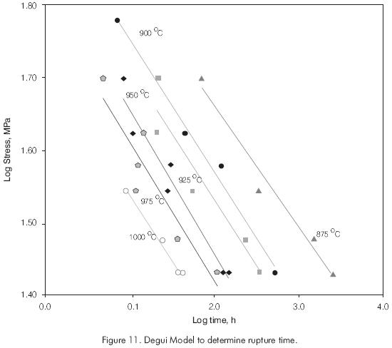
The values for the Degui model - chosen for being the one that comes closest to the experimental values and the differences between each of the results and the laboratory findings are included in Table 2. Figure 11 shows the tendency for the Degui model (equation 12) where the curves lead to a series of parallels to determine slope (b) and independent value (a). These would be: b = 0.182 y a = 1.83.
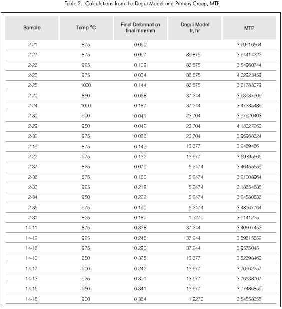
This model can be applied at temperatures greater than 1173K (900 °C), which represents 0.73 Tm (for the case of HK-40), with the disadvantage that predicts the same results for the same stress even when different temperatures are applied. Nevertheless, and limiting application to high temperatures, the model leads to an average deviation of 35% regarding the laboratory results (comparing the results shown in Table 1 with the data from this model registered in Table 2).
In the model proposed by Jasque and Simonen, constants Bi and ni from equation (7), which are functions of temperature, are found experimentally. The values for these constants vary, depending on temperature, from 2.8e-18 to 3.3e-7 for Bi and, from 11.14 to 2.48 for ni (temperatures between 1033K (760 °C) and 1363K (1090 °C), respectively).
According to Jaske and Simonen (1991), the results shown in Table 2 for the first phase can be obtained from equation (6). The idea is that this type of curves can be used to predict the behavior of the material at any state of stress and at a specific temperature.
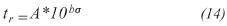
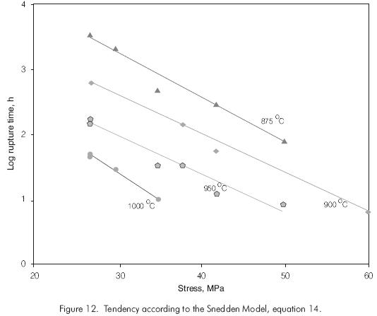
The Snedden model (equation 14) represents a series of quasi-parallel lines when the logarithm of rupture time versus stress is drawn. Slope (b) and the value of independent variable (A) can be determined from Figure 12. A value of b = - 0.0645 is obtained by applying the experimental results obtained Table 2 and A will be defined for each temperature. Nevertheless, as illustrated in the diagram Figure 12, the curves are not all that parallel, the behavior of the material is not very homogenous, which makes it difficult to apply this model predictively. This is very similar to what has been occurring with the other models.
General model proposed for the three stages of creep.
Based on the information found in the literature, the following model is proposed for application on the models and experimental data already described, to predict the general behavior of the material in creep conditions, in accordance with the principle of superposition:
E is the module of elasticity; q, p, m are constants; C1, C2 y C3 are the creep constants for the first, second and third stages respectively. s: applied stress. The other variables have already been defined in previous paragraphs.
The first term of equality (equation 15) is the elastic deformation, already defined in previous paragraphs and indicated in Figure 1 as ε0; this refers to the instant in which the sample is loaded to conduct the test of uniaxial stress on creep. Continuing with Figure 1, the three stages of visco-deformation can be observed. During the first stage, the curve acquires a decrease to a power (q, p) which will be εI. Then comes a steady state, that complies with Arrhenius. law and this will be εII (similar to equation (5)). Finally, there is an acceleration in deformation up until the rupture, εIII, which has an exponential form.
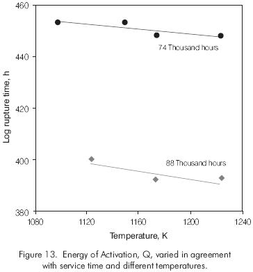
The activation energy, Q, can be found (if there is no known bibliographical data) by experimental means and simple calculation. To do this, tests are conducted at a uniaxial load, at a minimum stress and different temperatures; later, the data found are introduced into the following relation:
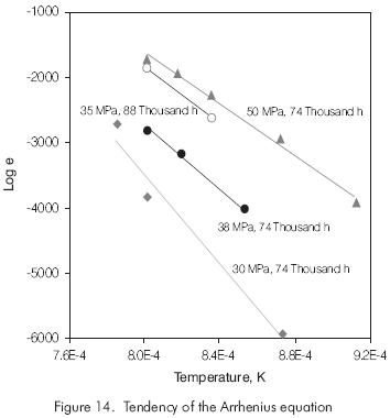
The graphic representation of this equation for the specimens chosen can be observed in Figure 13. The activation energy includes the damages and defects that the material might have. For the material worked up to 74 thousand hours, the activation energy will have a value of 450 kJ·mol-1, while for the material with 88 thousand hours of work, it will be 390kJ·mol-1 with a loss equivalent to 14% at a difference of 14 thousand hours. The damages and defects (dislocations, for instance) that occur inside the material during its servicing time are included in the change of activation. Figure 14 shows the curves for different stresses and for each aging time, applying Arrhenius. law used to find the third term in equation (15).
Illustrating the different values for each equation and those found experimentally (for effects of comparison, the results from sample 2-21, Table 1 are used here), the tendency of the curve can be observed in Figure 15, by using the following variables: T = 1148K (875 °C), σ= 27 MPa of applied stress, C1 = 0.5, C2 = 1, C3 = 0.05, C4 = 0.0041, m = 5, n = 11, p = 0.3, q = 1, R = 8.314 J·mol-1 K, Q = 450 KJ·mol-1.
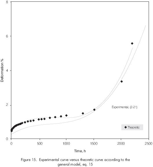
As can be seen, the theoretic curves (applying this model) and what has been found in the laboratory come very close, with a margin of error between 20 and 30%; this allows the prediction of the behavior of the materials at creep conditions. A disadvantage of this model is the amount of constants that must be found experimentally, which in the best of cases must be assumed. Therefore, the research continues to adjust the model, to reliably predict the useful life of the material in service.
CONCLUSIONS
-
The different models to predict rupture time have been discussed in order to determine the most appropriate one for the HK-40 material aged under service.
-
The Degui Model can be applied for high temperatures (T > 0.73Tm). This model has an average difference of 35% regarding that found in experimental tests.
-
The Larson-Miller model, varies from 40% to 50% in the prediction of rupture time, greater than that found in laboratory tests.
-
As far as tendency in rupture time, the Larson-Miller Model has a parallel tendency which indicates a nonconvergence as expected for this model.
-
The application of the Manson-Haferd Model tends not to converge, which disqualifies it to predict rupture time.
-
The Snedden Model presents a deviation in parallel behavior resulting in an increasing error regarding the prediction of rupture time.
-
The model proposed comes close to the experimental data. The margin of error is between 20 and 30%.
ACKNOWLEDGMENTS
The authors would like to acknowledge Javier Mateus from the Material Laboratory (ICP), for his constant support and collaboration during testing.
REFERENCES
API RP- 530, 1996. "Calculation of heater-tube thickness in Petroleum Refineries". [ Links ]
ASTM A-608, 1991. "Standard Specification for Centrifugal Cast Iron-Chromium-Nickel High Alloy tubing for pressure application at high temperature". [ Links ]
Courtney, T. H., 1990. "Mechanical Behavior of materials". Creep in Structures., 1997, http://pmlab.esm.psu.edu/class/215wll_2.htm. Creep in Metals, 1997. http://www.eng.wayne.edu/MSE130/creep.htm [ Links ]
Garofalo, F., 1965. "Fundamentals of creep and creeprupture in metals". [ Links ]
Iso Technical Report 7468, 1981. "Summary of average stress rupture properties of wrought steels for boilers and pressure vessels". [ Links ]
Jaske C. E., Simonen, F. A., 1991. "Creep-Rupture properties for use in the life assessment of fired heater tubes". [ Links ]
Latorre, G., 1998. "Fenomenología de la Termofluencia en materiales metálicos sometidos a altas temperaturas". Ecopetrol - Universidad Industrial de Santander. [ Links ]
Latorre, G., Correa, R., 1998. "Creep behavior of 25Cr-20Ni steel with more than 70 thousand hours of service". In print. [ Links ]
LeMAY, IAN., 1991. "Principles of mechanical metallurgy". University of Saskatchewan. Canada. [ Links ]
Manson, S.S., Ensign,C.R., 1971. "A specialized model for analysis of creep-rupture data by the minimum commitment, station-function approach". London. [ Links ]
Vamas Materials Databanks. 1997. http://yukige.nrim.go.jp/. [ Links ]
Viswanathan, R., 1989. "Damage Mechanisms and life assessment of high-temperature components", ASM International. [ Links ]

