1 Technology Cooperation Agreement: Ecopetrol S.A. - Instituto Colombiano del Petróleo, A.A. 4185 Bucaramanga , Santander , Colombia ; Universidad Industrial de Santander (UIS) -Petroseismic Group, Bucaramanga , Santander , Colombia. e-mail: karen_pachano@yahoo.com

2 Geophysical Group, Research Unit, Ecopetrol S.A. – Instituto Colombiano del Petróleo.

3 Universidad Industrial de Santander- Professor School of Petroleum Engineering. e-mail: carlos.piedrahita@ecopetrol.com.co

(Received Jun.15, 2005; Accepted Oct. 17, 2006)

ABSTRACT. This paper presents some fundamental concepts of seismic anisotropy specifically those which have hexagonal symmetry (ordinarily called transversely isotropic in geophysics jargon).

There were made calculations of phase and group angles at a planar interface separating an anisotropic media, using routines written in Matlab ® and Maple ® language. The slowness surfaces of the qP, qSV and SH wave, as well as the ray paths in these two media were also estimated.

Although only the simplest situations are discussed, this paper is useful as a first step in understanding the fractured media, because it contains examples, software routines, and a reviewing of the basic concepts and formulas of wave propagation.

Keywords: anisotropy, phase angle, seismic wave, ray path, wave propagation, symmetry, isotropy, group velocity, elasticity, mathematical model.

Con la ayuda de rutinas implementadas en Matlab ® y Maple ® , se calcularon los ángulos de fase y grupo en una interfase entre un medio isótropo y anisótropo, las superficies de lentitud de fase de las ondas qP, qSV y SH; así como la trayectoria de los rayos en éstos dos medios.

Aún cuando se analizaron las situaciones más sencillas, este artículo resulta útil como un primer paso para entender los medios fracturados, debido a que contiene ejemplos, rutinas y la revisión de los conceptos y fórmulas básicas de la propagación de ondas.

Palabras claves: anisotropía, ángulo de fase, ondas sísmicas, trayectoria del rayo, propagación de ondas, simetría, isotropía, velocidad de grupo, elasticidad, modelos matemáticos.

INTRODUCTION

One of the challenges in the oil industry has been the characterization of naturally fractured reservoirs using seismic data. To accomplish this goal it is necessary to find an adequate description of the physics of fractured rocks and its relationship to the observed wave propagation in seismic measurements.

Using technical computing routines, it was simulated the propagation of waves in two models, each of them consisting by two homogeneous layers separated by a planar interface. Based on the anisotropy parameters, it was calculated the phase and group angles, the slowness surfaces of the P and S waves, and the ray paths through these media.

In the numerical examples, the following configurations were used:

Model 1: isotropic-isotropic

Model 2: isotropic-anisotropic

THEORETICAL BACKGROUND

The mathematical description of the phenomenon related with the propagation of waves in an anisotropic media differs significantly from that in isotropic media. According to Cerveny (2001) the main characteristics of the waves when they propagate within an anisotropic media are:

a. The phase and group velocities depend on direction – anisotropy.

b. There is a difference between the phase velocity (propagation of the wave) and the group velocity (propagation of energy).

c. Occurs shear wave splitting.

d. Polarization of the P wave is not strictly parallel to the direction of propagation (Quasi P).

e. Polarization of the S wave is not strictly perpendicular to the direction of propagation (Quasi S).

Elastodynamic theory

Continuum Mechanics is the starting point to describe the elastic properties of solids (Mase, 1970). Its major hypothesis is the infinite divisibility of matter and this assumption is valid for models at macroscopic level, so that the elasticity of a material is a macro property.

From Continuum Mechanics, specifically the Linear Elasticity Theory, it can be obtained the relationships ( Equations 1 and 2 ) that model the behavior of a body when deforming:

1. Moments and Forces balance

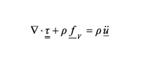
(1)

2. Generalized Hooke's Law

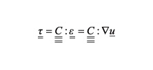
(2)

Where:

= force tensor

? = density

= volumetric forces

u = displacement vector

= fourth order elastic coefficient tensor

= deformation tensor

ü = aceleration.

Note: a vector will be differentiated with one underline, a tensor of second order with two underlines, and similarly the elastic coefficient tensor will have four underlines.

On the other hand, the microscopic characteristics of solids, such as the crystalline structure, are closely related to the macro behavior of an object under the influence of a stress field.

In seismic, the word anisotropy has to do with the resolution of the method employed to study the elastic properties of a particular object or of a global, macroscopic anisotropy that results from homogenizing the properties of the layers that form a laminated structure (i.e. effective medium).

The reason for introducing this new concept is that, in practice, the object being studied is formed from an initial background which originally was homogeneous (whether isotropy or anisotropy) and with time it acquires cracks faults, layers, etc., which changed the initial elastic properties. For example, an isotropic medium could have the anisotropic elastic characteristics with the presence of aligned cracks or layers.

From Equations 1 and 2 it can be obtained the general elastodynamic equation for homogeneous media, which is the fundamental basis for modeling the propagation of waves:

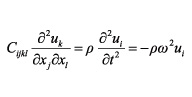
(3)

In Equation 3

C_ijkl = Elastic coefficients tensors (constant for homogeneous media)

u_i = Displacement vector

? = density (constant for homogeneous media)

? = angular velocity

x_i = spatial coordinates

t = time

A plane-wave solution of the elastodynamic equation is found as follows: (A more general solution can be obtained using the so called high frequency approximation, or ray theory, it supposes a solution of the wave equation of the form of Equation 4 but, with amplitude and travel time varying with space).

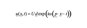
(4)

Where:

U = constant of integration (Amplitude)

d = polarization vector

p = slowness vector

x = spatial coordinates

t = time

Substituting the expression (4) into the Elastodynamic Equation, we arrive at the Christoffel Equation:

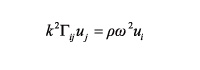
(5)

Where:

G_ij = Christoffel's Matrix.

The Christoffel Equation has non-trivial solution only when the determinant of the characteristic matrix is equal to zero, namely:

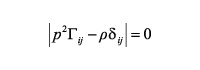
(6)

To resolve the Christoffel Equation is the same as finding the eigenvectors and eigenvalues to the matrix that carries the same name. These may be obtained if the matrix of elastic coefficients is known, as well as the wave propagation direction vector, through the following formula:

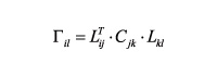
(7)

Where:

G_il = Christoffel's Matrix.

L_ij – Matrix of director cosines of the propagation vector.

C_jk – Matrix of elastic coefficients in the Voigt form.

Anisotropy and fractures

Many theoretical and experimental studies have been carried out to try and explain the behavior of the seismic waves when they travel through fractured media (Crampin, 1980; Hudson, 1980; Schoenberg & Sayers, 1995).

According to laboratory tests and evidence, it has been concluded that when the seismic waves propagate through fractured a media, the following occurs: low velocities, high attenuation, and changes in the velocities with the propagation direction (Crampin, 1980; Chen, 1995; Rüger, 1997).

The presence of fractures (generally vertically aligned microcracks generated by tectonic forces) makes the medium anisotropic with respect to wave propagation (Schoenberg & Douma, 1988). Even though the presence of azimuthally anisotropy has great influence on all the propagation modes (P, S Waves), the existing studies concentrate on analyzing the delay of the reflective amplitudes of splitting S waves (S1 and S2).

According to the theory, the orientation of the fractures can be determined by the division of the S wave (shear wave splitting). Polarization of the rapid S wave (S1) is parallel to the fractures and the slower propagation of the S wave (S2) is perpendicular to the fractures (Crampin, 1980; Evans, Gaucher, & Randall, 2000).

It was recently demonstrated that the azimuthal dependence of the characteristics of the P waves, has the power to determine the orientation and intensity of the fracture system (Bakulin, Grechka, & Tsvankin, 2000; Rüger & Tsvankin, 1997; Garnica, 2003).

In summary, in order to study the fractures with reflection seismic data, it is essential to combine several disciplines, among them seismic anisotropy, rock physics and seismic methods (Figure 1).

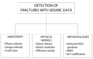
Figure 1. Disciplines involved in detecting fractures with seismic data

As stated before, the matrix C_ij (in Voigt notation) represents the elastic coefficients. They define the behavior of the continuum media. If the continuum is symmetric at some coordinate changes, it is possible to enunciate those coefficients according to their symmetries, and at the same time, reducing the number of independent terms.

Table 1 illustrates the type of symmetry that can have a solid and the number of elastic constants needed to describe its behavior.

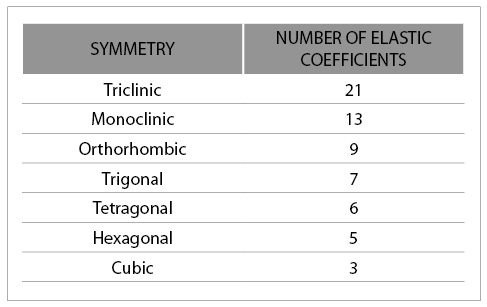
Table1. Number of elastic coefficients according to its symmetry

The continous media that presents a hexagonal symmetry are commonly called “transversely isotropic”, these have the invariant elastic properties in two of the three axis (isotropic plane).

The simplest anisotropic models that can be used to represent fractured reservoirs are Transversely Isotropic (TI) media. According to the orientation of the symmetry axis, the TI media can be Transversely Isotropic with a Vertical axis of symmetry (VTI) or Transversely Isotropic with a Horizontal axis of symmetry (HTI).

Examples of VTI media are systems with lamination or stratification, such as the sequences of shale, chalks and clays, commonly found in the sedimentary basins. Consequently an HTI medium would be represented by a set of parallel fractures imbedded in an isotropic matrix.

A model that could represent the fractured reservoirs in a more realistic way is the orthorhombic medium, in which we can observe layers or strata (VTI) intersected by a set of vertical fractures. The complexity of this system is based on the number of elastic coefficients that are necessary for its description (Table 2).

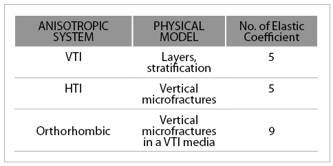
Table 2. List of the anisotropic systems and elastic coefficients

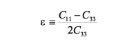
The mentioned models (VTI and HTI) are the simplest case of anisotropy and they can be represented by five elastic coefficients. In 1986, Thomsen used three dimensionless parameters e, d, y ?, and vertical velocities of the P and S waves.

The dimensionless parameters represent the influence of the anisotropy on several seismic characteristics, under the context of the weak anisotropy, which apply to geologic formations where Thomsen?s parameters are less than 20 percent (20%).

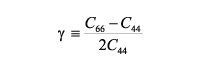
According to Thomsen, the physical meaning of the parameters e, d, ? is as follows:

e: is the fractional difference between the velocity of the horizontal and vertical P waves, defined in terms of elastic constants as:

(8)

?: is the fractional difference between vertical and horizontal velocities (the difference between the shear velocity for polarization parallel to the symmetry planes in polar anisotropy and vertical shear velocity).

(9)

d: is the variation of the P wave with the phase angle.

(10)

(11)

The C_ij constitutes the matrix of elastic coefficients.

NUMERICAL EXPERIMENTS

Calculation of phase and group angles

The phase and group angles are calculated following the methodology outlined by Slawinski (1996). See Appendix A.

The assumptions taken into account for this calculation are:

• Weak anisotropy

• Macro scale (presence of cracks, discontinuities, fractures)

• Longitude of long wave

• Low frequencies (geophysical context)

• VTI Symmetry (5 elastic coefficients)

The configurations of the models are as follows:

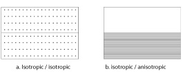
Figure 2. Used configurations.

Table 3 shows input data to calculate the phase and group angles from the incidence angle between the isotropic and the anisotropic media.

According to those examples, it can be stated that the elastic parameters for an isotropic media correspond to a homogeneous medium (also called continuous media) where there is no fractures, microfractures or cracks, as it is true in consolidated rocks.

The elastic parameters for the isotropic medium were measured in consolidated rocks without fractures or cracks.

On the other hand, the elastic parameters for the anisotropic media correspond to rocks with cracks, cavities or discontinuities.

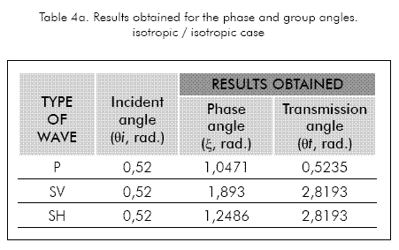
Tables 4a and 4b show the results obtained for the configuration isotropic / isotropic and isotropic /anisotropic respectively.

Slowness surfaces

Once we have the elastic coefficients we proceed to plot the slowness surface (inverse of the phase velocity), which is obtained by solving the Christoffel Equation (Equation 5), Duarte et al., 2004.

Figures 3, 4 and 5 represent the slowness surfaces for each wave.

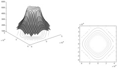
Figure 3a. Slowness surface for the P wave.

Configuration isotropic / isotropic

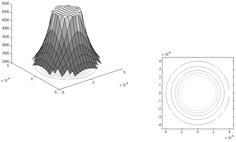
Figure 3b. Slowness surface for the qP wave.

Configuration isotropic / anisotropic

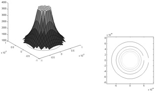
Figure 4a. Slowness surface for the SV wave.

Configuration isotropic / isotropic

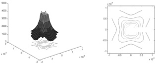
Figure 4b. Slowness surface for the qSV wave.

Configuration: isotropic / anisotropic

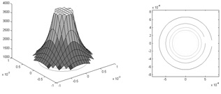
Figure 5a. Slowness surface for the SH wave.

Configuration: isotropic / isotropic

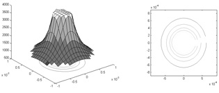
Figure 5b. Slowness surface for the qSH wave.

Configuration: isotropic / anisotropic

Ray tracing in anisotropic media

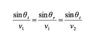
Ray tracing is based on Snell's Law. In the isotropic case, where the velocities of phase and group coincide, Snell's Law has a simple representation.

(12)

In the anisotropic case, the representation of Snell's Law is more complicated. Figure 6 shows the geometric interpretation.

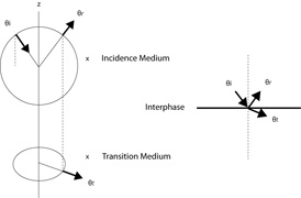
Figure 6. Geometric representation of Snell's law (Slawinski, 1996)

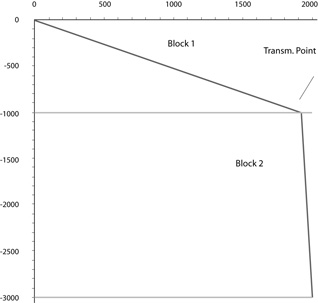
Figure 7. Path of one ray in a medium composed of two blocks, each one with the elastic properties of the isotropic media

According to Figure 6 in the case of anisotropy: ?_i , ?_r , and ?_t , represent the angles of incidence, transmission and reflection for the slowness vectors respectively. The ellipses are the slowness surfaces for each of the media.

The model considered has two layers, the first one is isotropic and the other one is anisotropic. The independent variable to be found is the horizontal distance r between the first transmission point to the receiver. The variable r was calculated using the following equation: (Slawinski, 1996).

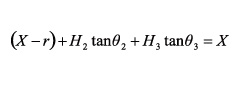
(13)

Equation 13 is easily generalized for a model of multiple layers only by adding the sums of type H_k tan? k for each of the additional layers. The problem is reduced to find transmission angles ?_k in terms of the independent variable r.

First we find the departure angle and the ray parameter x:

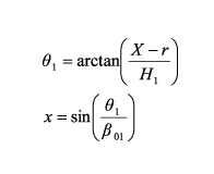
(14)

Here, x is the ray parameter and ß₀₁ is the vertical phase velocity for layer 1. The phase and group angles are calculated for each of the layers. For example, the f₂ phase angle for layer 2 is as follows:

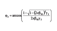
(15)

Where ß₀₂ is vertical phase velocity for layer 2 and ? 2 is the Thomsen parameter for the same layer. The group angle is found as follows:

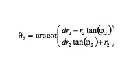
(16)

Where r₂ y dr₂ are intermediate variables:

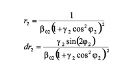
(17)

Figures 7 and 8 show the path of the ray in the isotropic/isotropic and anisotropic/ anisotropic cases.

ANALYSIS OF RESULTS

With Figures 3, 4 and 5 it is possible to corroborate the dependence of the phase slowness (inverse of the phase velocity) with the direction.

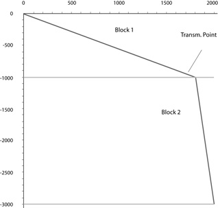
Figure 8. Path of one ray in a medium composed by two blocks. The properties of the upper block are isotropic and the properties of the lower block are anisotropic

In isotropic media the direction of the SV and SH wave is the same (transmission angle).

Comparing the rays obtained with the isotropic/isotropic and isotropic /anisotropic configurations (Figures 7 and 8); a horizontal displacement is observed from the transmission point of the ray between blocks 1 and 2. For this reason if the anisotropy of the medium is not taken into account, a different transmission point will be calculated, thereby generating errors in the calculations of travel time.

DISCUSSION

In this paper was presented the foundations for the understanding of the wave propagation in anisotropic media. Although it was presented the simplest case, it is a good starting point in the analysis of seismic velocities having the whole theory behind the phenomena, and some numerical examples.

In order to properly simulate the wave propagation phenomenon in a complex medium, it is necessary to know its elastic properties as well as its anisotropic parameters, particularly for samples with cracks, cavities or discontinuities.

ACKNOWLEDGEMENTS

The authors express their gratitude to: Instituto Colombiano del Petrsleo (ICP) of Ecopetrol S.A. and to the Universidad Industrial de Santander (UIS), for sponsoring the development of this research.

REFERENCES

Bakulin, A., Grechka, V., & Tsvankin, I. (2000). Estimation of fracture parameters from reflection seismic data – Part I: HTI model due to a single fracture set. Geophysics, 65 (6): 1788-1802.         [ Links ]

Cerveny, V. (2001). Seismic Ray Theory. Cambridge University Press.         [ Links ]

Chen, W. (1995). AVO in Azimuthally anisotropic media fracture detection using P-Wave data and seismic study of naturally fractured tight gas reservoir. Ph. D. Thesis. Department of Geophysics, School of Earth Sciences, Stanford University, Stanford, California, 143 pp.         [ Links ]

Crampin, S. (1980). A review of wave motion in anisotropic an cracked elastic media. Wave motion, 3: 343-391.         [ Links ]

Duarte , M., Piedrahita, C., Salinas , T., Altamar, H., & Pachano, K. (2004). Slowness surface calculation for different media using the symbolic mathematics language Maple ®. Earth Sciences Research Journal, 8 (1), 63-67.         [ Links ]

Evans, R., Gaucher E., & Randall, N. (2000). Borehole seismic supplying answers to fractured reservoir questions. SPE 58994.         [ Links ]

Garnica, M. (2003). AVOA analysis and fracture characterization: Clair Field, West of Shetlands. M. Sc. Thesis. School of Earth Sciences , The University of Leeds , Leeds , England , 90 pp.         [ Links ]

Hudson, J.A. (1980). Overall properties of a cracked solid. Math. Proc. Camb. Phil. Soc., 88: 371-384.         [ Links ]

Mase, G.E. (1970). Theory and Problems of Continuum Mechanics. Schaum's Outline Series, McGraw-Hill.         [ Links ]

Rüger, A. (2002). Reflection Coefficients and Azimuthal AVO Analysis in Anisotropic Media, Geophysical Monograph Series. SEG - Society of Exploration Geophysicists, 10: 189 Tulsa , OK .         [ Links ]

Rüger, A.,& Tsvankin I. (1997). Using AVO for fracture detection: analytic basis and practical solutions. The Leading Edge, 1429-1434.         [ Links ]

Schoenberg, M., & Douma, J. (1988). Elastic wave propagation in media with parallel fractures and aligned cracks. Geophysical Prospecting, 39: 571-590.         [ Links ]

Schoenberg, M., & Sayers C. (1995). Seismic anisotropy of fractured rock. Geophysics, 60 (1): 204-211.         [ Links ]

Slawinski, M.A. (1996). On elastic-wave propagation in anisotropic media: reflection/refraction laws, ray tracing, and traveltime inversion. Ph. D. Thesis. Department of Geology and Geophysics. The University of Calgary , Calgary , Alberta . 223 pp.         [ Links ]

Thomsen, L. (1986). Weak elastic anisotropy. Geophysics, 51 (9): 1954-196         [ Links ]