Saúl-Ernesto Guevara-Ochoa¹ and Peter William Cary²

¹ Ecopetrol S.A. – Instituto Colombiano del Petróleo, A.A. 4185 Bucaramanga , Santander, Colombia. e-mail: sguevara@ecopetrol.com.co

² Sensor Geophysical, Canada

(Received June 15, 2005; Accepted Dec. 5, 2006)

ABSTRACT. The multicomponent (3C) seismic method is an emerging technology, which allows recording the complete wave field, including converted (PS) waves. Methods to obtain information about fractured rocks have been developed from these data since anisotropy, an effect of parallel fracture trains, generates birefringence of PS waves. We present here an application of this technology to data from an experimental seismic survey from a setting of NE Colombia. The geological characteristics of this setting were challenging for the current processing methods. A 3C seismic line following geological strike and another one following dip were processed. Coherent noise statics correction and velocity analysis required an iterative approach. The presence of polar anisotropy related to stratification, was taken into account for stacking. This approach greatly improved the resulting section, verifying its suitability.

Three seismic sections, each one corresponding to a component, were obtained for the strike line. An azimuthal anisotropy analysis was carried out on them. Significant results were found, that might imply the presence of natural fracturing directions. This result requires to be tested with complementary geological information.

About the dip line processing, the method applied appear unsatisfactory. There were identified shortcomings of processing related to dipping strata and complex structures, which became worse by the noisy data. More advanced processing methods would be required in this case.

Keywords: fractures reservoirs, seismic method, p-wave, s-wave, anisotropy, anisotropy means.

RESUMEN. El método sísmico multicomponente (3C) es una tecnología emergente que permite registrar todo el campo de onda, incluyendo las ondas convertidas (PS). Se han desarrollado métodos para obtener información acerca de las rocas fracturadas a partir de estos datos, ya que la anisotropía azimutal, un efecto de los trenes paralelos de fracturas, genera birrefringencia en las ondas PS. Aquí presentamos una aplicación de esta tecnología a datos sísmicos experimentales obtenidos en un sitio al Nordeste de Colombia, cuyas características geológicas son retadoras para el estado actual de los métodos de procesamiento. Se procesaron dos líneas sísmicas, una siguiendo el rumbo de las estructuras geológicas y otra siguiendo el buzamiento. El filtramiento de ruido coherente, la corrección estática y el análisis de velocidad requirieron de un enfoque iterativo especial. Se tuvo en cuenta la presencia de anisotropía polar, relacionada con la estratificación, en el proceso de apilamiento, con lo cual se mejoró la sección resultante, verificando así la ventaja de ese modelo.

Para la línea de rumbo se obtuvieron tres imágenes sísmicas, una correspondiente a cada componente. Con base en ese resultado se hizo un análisis de anisotropía azimutal, en el que se obtuvieron resultados significativos. Estos resultados podrían implicar la presencia de direcciones de fracturas naturales, las cuales requieren de información geológica complementaria para su verificación.

Con respecto a la línea de buzamiento, los métodos de procesamiento no fueron satisfactorios. Se identificaron limitaciones relacionados con los estratos bufantes y las estructuras complejas, las cuales se agudizan en la presencia de datos ruidosos. Se requieren métodos más avanzados en este caso.

Palabras clave: yacimientos fracturados, métodos sísmicos, ondas p, ondas s, anisotropía, medio anisotrópico.

INTRODUCTION

The multicomponent seismic method allows recording the complete wave field by using three components (3C) sensors, which are sensitive to the wave displacement vector. Vibration of Shear (S-waves) reflected at geologic interfaces are close to horizontal at the earth surface, consequently can be detected with this method. S-waves are sensitive to anisotropy (e. g. Crampin, 1985), since they are vectors. Converted waves are a type of S-waves. As natural fractures are considered a cause of anisotropy, it would be possible to obtain information about fractures using converted waves. The subject of this paper is the application of this method to a data set of a geologically complex area in the Northern Andes of South America.

There are many unknowns about the characteristics of naturally fractured reservoirs even though it is considered that they can constitute a significant share of oil reserves (Aguilera, 1998), particularly in Colombia (e.g. Villamil, 2001). Well logs and rock sample analysis from cores yield reliable and detailed information about local characteristics. The missing data (the “big picture”) should be provided mostly by educated geological inference. Seismic data can fill the gap between these two kinds of information, since with this method it is possible to obtain a full image of 2D earth cross sections and 3D volumes. Seismic resolution is about tens of meters (e. g. Winterstein, 1992), much coarser than wells information, however it is statistically meaningful, and can contribute with fundamental information to support a fractured geological model.

Natural fractures are generally found in orientations determined by rock properties and their stress story, which originate properties associated with direction, that is to say, anisotropy. Two anisotropical relatively simple models have been useful in practical applications. Vertical parallel fracture trains is a simplified model of fractures in the earth's crust. Corresponding to this geometry there is a theoretical anisotropy model known as azimuthal anisotropy or HTI media (Horizontally Transverse Isotropy). Another anisotropycal model of practical interest resembles geological stratification. It is known as polar anisotropy or VTI (Vertical Transverse Isotropy) media, which can be related to horizontal parallel sediment settling (Thomsen, 2002).

The relationship between anisotropy and wave propagation has been subject to active research. As mentioned before, S waves are sensitive to fracture orientation. S wave polarization depends on the relationship between the propagation direction of the wave, and the direction of the fracture train (Winterstein, 1992). The different properties in two orthogonal directions generate birefringence of S wave, that is S wave splits into two modes, a fast one and another slower, the former corresponding to fracture direction polarization (Crampin, 1985). The azimuthal variation of properties caused by anisotropy, according to the HTI model, also affects P wave characteristics with azimuth, such as reflections arrival time, and amplitude with the angle of incidence (Thomsen, 2002).

A number of seismic techniques have been developed to detect anisotropy related to fractures, taking advantage of the properties just mentioned. Some of these techniques use polarizacisn of S waves and other use azimuthal properties of 3D P-waves. Two methods which take into account azimuth changes in P wave seismic data. One of them uses the NMO (Normal Move Out) velocity analysis with azimuth for 3D data, that is arrival times for a CDP (e. g. Thomsen, 2002), and the other method uses the AVO (Amplitude Variation with Offset) effect with azimuth (see R?ger and Tsvankin, 1997). In order to analyze these type of properties, 3D data of P waves with a broad azimuth distribution is required.

P-wave 3D is a robust and extended technology, but its sensitivity to fractures appear lower than S-waves (Thomsen, 2002). Pure S-wave, despite being more sensitive, lacks good energy content in general, among other processing shortcomings. Converted waves appear as a promising option with benefits compared to the other techniques. Converted or PS wave (also as C wave) has been subject of great interest (e. g. Stewart, Gaiser, Brown, & Lawton, 2002; Thomsen, 1999; Garotta, 2000) by its information content, energy content and easier generation compared to other wave modes. However its application has been limited, since some related techniques like processing are not well developed and demands quite good data quality.

Applied works using converted waves to detect fracture properties have been more successful in seismic data with a high S/N ratio and at settings with relatively simple geological characteristics. An example is the work presented by Ata and Michelena (1995).

The work presented here illustrates the application of this technique to data originated in Northern Colombia, a zone affected by the tectonic processes of the Andes Mountains of South America. Shortcomings to handle the complex geometry are identified. Anyway meaningful birefringence analysis of the strike line could be performed, showing the potential of this method to indicate potential fracture directions.

This paper begins with a brief description of the methodology for fracture analysis; after that there is information about the geological setting and the seismic data characteristics; then details of the processing; and finally the birefringence and fracture analyses.

METHODOLOGY

Figure 1 illustrates the model of birefringence that explains the effect of fracture trains on S wave. It involves wave field displacement direction or polarization , which is detected by the multicomponent seismic method.

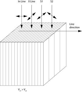
In the 2 D multicomponent method, one of the two horizontal components follows the line direction, and it is called radial or in-line; the other one is perpendicular to it, and it is called transversal or cross-line. In principle, according to an isotropic model, converted wave in a plane oscillate in the source-receiver direction, identified as in-line in Figure 1. If there is azimuthal anisotropy, such as the one that might be generated by fractures, two S waves, identified as S1 and S2 are generated by a birefringence effect. S1 wave is faster and it is polarized in a direction parallel to fractures, and the S2 wave is slower and it is polarized perpendicularly to fractures (Figure 1).

Several azimuthal anisotropy analysis methods that use S waves have been developed. For converted waves, a cross-correlation method, was proposed by Harrison (1992). Garotta (2000) also provides a description of the principles of this method. This method was applied in this work.

This method models the cross-correlation of the radial and transverse components as a function of time delay and azimuth angle. The resultants of the two horizontal components rotations are calculated and cross correlations are made between them for each rotation angle. In a highly simplified sense, Harrison's method works by trying to find the azimuth and time delay parameters that make the wavelets in the real data match the behavior of a synthetic pair of wavelets that have a specific polarization direction and delay time. It is very important with Harrison's method that the input data be processed in a true relative amplitude fashion so that the relative differences are preserved in the data. Experience with Harrison's algorithm has shown that the results are sensitive to the presence of noise-especially coherent noise-on one or both components. Therefore it is best to use stacked data as input to the algorithm.

The result of the correlations is presented graphically for each rotation angle values and each displacement and high correlation values must be found for the dominant displacements and the dominant polarization directions, as will be shown in the fracture analysis section.

DATA CHARACTERISTICS

Study area and the seismic data

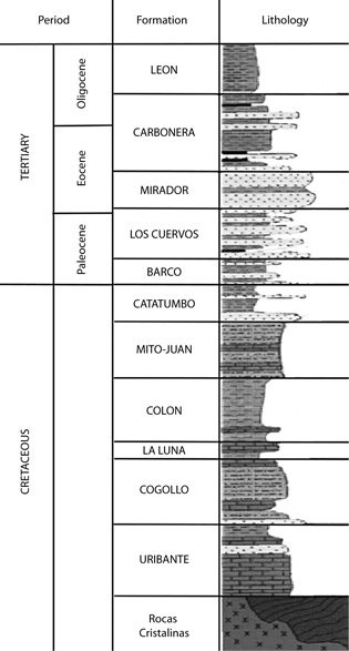
The Catatumbo area, in Northeast Colombia, has potential of hydrocarbons in naturally fractured rocks. Figure 2 shows a generalized geological column of this area. The rock formations originate mostly at the Tertiary and the Cretaceous. Sandstones and shales predominate in the Tertiary and, calcareous rocks, shales, and limestone in the Cretaceous. Cretaceous calcareous formations can contain fractured reservoirs.

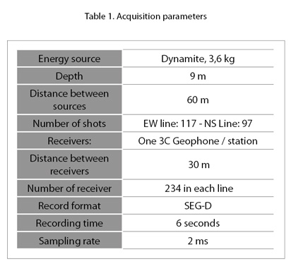
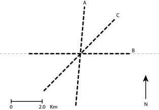
Three multi-component seismic lines were acquired in this area in the year 2000. Table 1 shows the acquisition parameters. The location and direction of the seismic lines is illustrated in Figure 3. with the lines identified with letters A, B, and C. Each one has 7 km length, and cross each other at its center. Lines identified with letters A and B in Figure 3, are approximately orthogonal to each other.with distance between receivers of 30 m. The line A, with approximately NS direction, follows the strike of the geological structure, and the line B, with EW direction, follows the dip. The complete spread was activated throughout all the recording time of these two lines thus generating a “pseudo” 3D dataset. This work is focused on these two lines. Line C was shot independently, and its distance between receivers was 15 m.

Field record characteristics

As a first approximation, the vertical component can be considered equivalent to P wave and the radial component to PS (or converted) wave. The transversal component could contain out-of-the–plane events, or events related to birefringence.

These assumptions can be considered by its statistical meaning, since probably large offset traces could include non vertical incidence, or mispositioned geophones could include converted waves in the transversal component. A test of these assumptions will be shown further, on the processing results and fracture analysis, which confirm them. However the vertical incidence assumption can be also justified by the increase in velocity with depth, which refracts the wave fronts (Yilmaz, 1987, Tatham & McCormack, 1991). For a case of constant velocity the maximum angle of incidence would be 30° (according to the maximum offset and the target depth), for velocity increasing with depth it would be reduced, and it would be closer to 0° for shorter offsets. In fact, usual velocities for P-waves at the near surface layer in this terrain are lower than 1000 m/s, which has a noticeable contrast with the hard rock, whose velocity use to be around 2000 m/s or higher, so we would have an angle of incidence to the surface of about 14° as a maximum. Even more pronounced contrast can be found for shear waves (Tatham and McCormack, 1991). Finally, as the processes applied select events by velocity analysis and stacking, the possible converted waves in the vertical component and P-waves in the horizontal most probably are removed out, which contributes to obtain results according to the assumption.

Figure 4 illustrates typical field records for each of the three components, vertical (Figure 4a), radial (Figure 4b), and transverse (Figure 4c). Several seismic events, identified with numbers, can be identified in these records. It allows the next interpretation:

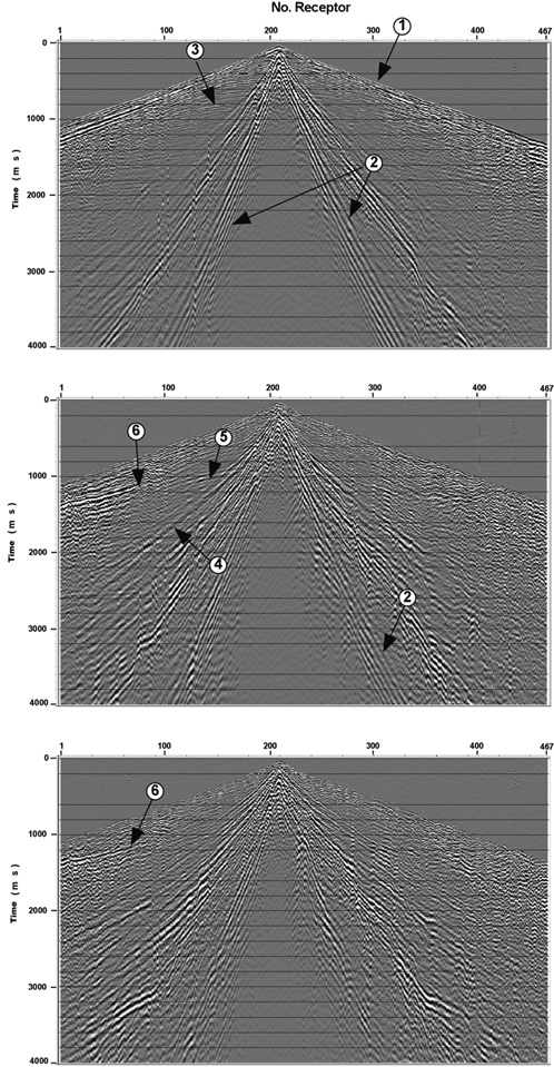
1. First arrivals, mainly P wave refractions.

2. Surface waves (ground-roll).

3. P wave reflections.

4. Probably PS wave refractions.

5. PS mode reflections and

6. PS reflections beyond the critical angle.

Identification of these events allowed confirming the correlation of recording channels and components with the orientation of detectors on the surface. P wave information on the vertical component shows enough energy content and clear reflectors. The converted wave is also distinguished on the radial or in-line component, even perhaps less clearly.

Effect of the near surface (statics) can be observed in the horizontal components (Figures 4b and 4c), when compared to the vertical component. It can be also observed that horizontal components have a smaller reflectors window than vertical component due to the presence of coherent noise. This is a shortcoming for converted waves since they are slower and arrives later.

DATA PROCESSING AND RESULTS

Strike line processing

Figure 5 illustrates the processing flow for converted waves. On line A radial and transverse sections of PS wave could be obtained, and later on, fracture analysis could be carried out, which was not possible on line B. Likewise, 3D data of the vertical component (P wave), resulting from the simultaneous activation of lines A and B did have appropriate azimuthal angles to perform an anisotropy analysis with the aforementioned P wave methods, hence this option was discarded.

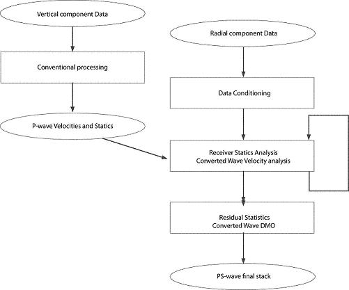
Figure 5. Simplified PS-wave multi–component processing flow chart

Figure 6 shows the result of the line A vertical component processing, along with the corresponding geological interpretation. This procedure was straightforward without major problem.

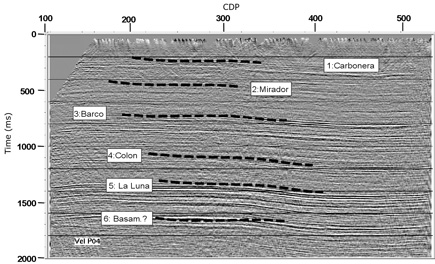
Figure 6. P wave section (vertical component) final binning. Line A The interpretation of the main horizons is indicated

As shown in Figure 5, the radial component data requires to be conditioned first, which in this case meant basically noise attenuation. Source static correction was taken from P wave processing, and receiver statics (for S wave) required an specific procedure. Statics correction and stacking velocity analysis were critical steps regarding the processing of these data. After that a DMO algorithm (Harrison, 1992) was applied. Additionally to the steps described in Figure 5, the effect of VTI anisotropy was taken into account during the stacking step. Also factors altering amplitude, regarding a vector analysis of the horizontal components were taken into account. In order to perform the birefringence analysis correctly with the method proposed, it is necessary amplitude consistency in processing of horizontal components. Amplitudes should be consistent to the surface, so special care must be taken regarding the processes affecting them such as deconvolution.

The main interference on these data was the coherent noise originating in the surface waves or ground-roll, which affects PS wave to a greater degree (Figures 4b and 4c). Filtering applied separately to positive and negative offsets was used in the fk domain (Yilmaz, 1987), which rendered a result with enough quality to allow proceeding on to subsequent stages.

Statics correction has been recognized as important issues in converted wave processing (Anno, 1986; Tatham, & McCormack, 1991), since conventional methods such as refractions and residual statics do not work appropriately. As seen in Figure 5, source statics, since corresponds to P wave, was taken from the vertical component processing. A modified version of the method proposed by Cary and Eaton (1993) was used here for the receiver statics correction. This process is carried out in the common receiver gather domain. The total delay time for each trace can be represented as follows (Wiggins, Larner, & Wisecup, 1976):

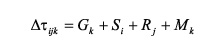
(1)

Where S_i is the source static correction at source i, R_j is the receiver static correction at receiver j, G_k represents the structural component (delay time related to Geology), and M_k is the NMO effect on CDP k. This implies that, in order to obtain receiver statics, NMO correction, statics correction of the source, and correction of the effect caused by the geological structure should be known. Thus, since the source statics corrections and the geological structure are both known, assuming an event whose structure is smooth enough, an iterative receiver statics and NMO correction process is defined. The detailed process is as follows:

1. The best available processing parameters are applied to previously binned data. The signal is highlighted according to available parameters (noise filtering, band pass filter, etc.)

2. Source statics correction is applied.

3. Stacking is obtained in the receivers dominion Common Receiver Stack (CRS), with NMO corrected data. Receiver statics is corrected on these data, which means maintaining structural geological characteristics, and every additional offset would be an effect caused by statics.

4. A new velocity analysis is performed, and a loop is made back to number 3 until a satisfactory stacking is obtained.

Velocity analysis (Step number 4) is a critical stage of this procedure. In the case of converted waves, we have an asymmetric raypath. This asymmetry depends on the physical properties of the rock, as expressed by wave velocity (Tatham & McCormack, 1991). This leads us to a looping problem, since, in order to find the right velocities and stacked sections, physical properties must be known, and vice versa. This explains partially the need to perform an iterative process at this point. VTI anisotropy, which is related to stratification, will be considered further on.

Results of receiver statics correction are illustrated in Figure 7, as compared with receiver statics for the vertical component (P wave). It can be seen that the radial component statics has a 90 ms range, much larger than the vertical component range, which is 20 ms.

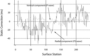
Figure 7 Statics corrections for the NS line receiver

The velocity analysis also had some issues to be considered. A common strategy toward the analysis of converted wave is finding adequate values for the V_p /V_s relationship, so that it can be possible that, from the velocity field resulting from vertical component V_p processing, the velocity field of the converted wave can be obtained. We can identify this relationship V_p /V_s from this point on, with the symbol y (Greek letter Gamma).

Here, a different strategy was used: the best possible image was sought from the converted wave, by exploring stacking velocity for radial component data. By this way the resulting stacking velocity is a “compound” velocity, partly V_p , and partly V_s, called V_c by Thomsen (1999). Since this velocity is independent from the resulting from P-wave processing, this is an additional data entry which can be used within the analysis later on. Considering the low signal – noise relationship in these data, velocity analyses were performed using constant velocity stacks. Several velocity – statics iterations were required in order to obtain a satisfactory result.

Based upon the interpretation of this line's events in the P wave section illustrated in Figure 6, a corresponding interpretation was made on the most remarkable events in the converted wave section. The procedure for such correlation was using events which are distinguishable because of their energy contents and their character. The reflector identified by number 5 on Figure 6, top of La Luna Formation was identified as being the most characteristic event. After that, taking into account the arrival time, and assuming a 2,0 V p /V s ratio, the other reflectors were identified. The final result of this interpretation is presented in the converted wave section of Figure 8.

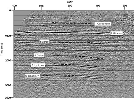
Figure 8. Interpretation, wave PS, line A

The final result of this velocity analysis is shown in Figure 9, where stacking velocity for P wave (vertical component) is compared with radial component velocity (V_c). In this figure, for comparison purposes, both velocity fields are presented as a function of time for the converted wave section (Figure 8 and Figure 6). To this end, P velocity values were converted to equivalent time in the converted wave section, calculating an appropriate ratio from the identification of corresponding geological events in the interpretation of the two images.

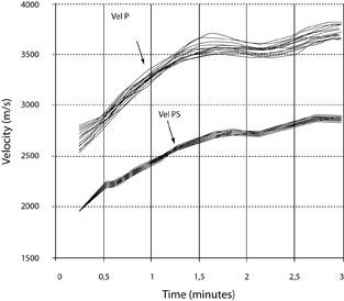
Figure 9. Comparison between P wave velocities and converted wave velocities

As it was mentioned above, the gathering process for the stacking traces in converted waves depends on the actual physical characteristics of the wave propagation velocity, such as it cannot be assumed from simple geometric characteristics, as it happens with P wave. One of these actual geological characteristics is anisotropy. In this case, the influential factor is layering, and consequently the polar anisotropy or VTI model can be applied. Thomsen (1999) defines the effective V_p/V_s ratio (Y_eff), as :

(2)

where Y_eff, is a function of two V_p/V_s ratios, namely y0 and y₂. Which takes into consideration the effect of the difference between horizontal and vertical velocities caused by such layering, since that parameter is derived from the parallel strata anisotropic model for the case of converted waves. The traditional value, represented here as y0, is related to vertical velocity, which would correspond to the ratio between times for zero – offset events. The other value, y₂, is the stacking velocity ratio for short offsets, defined as offsets shorter. Thus, we will have the following ratios:

(3)

where V_P2 and V_S2 correspond to stacking velocities for short offsets. In a practical sense, this relationship Y_eff can be defined as the one that allows to obtain the best CCP stacking, since yields a better gathering.

Thus, a series of tests was performed for several Y_eff, values, and the best stacking was obtained for Y_eff ratio of 1,5. The resulting stacked section is shown in Figure 10 which shows improvement if it is compared to Figure 8.

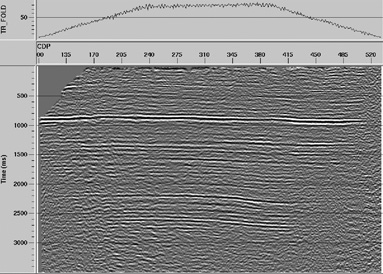
Figure 10. CCP stacking using 1,5 effective Vp/Vs and f-x deconvolution

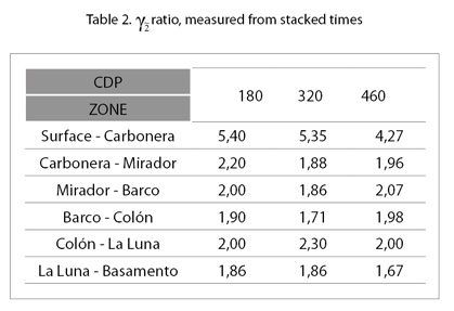
Tabla 2 shows values for y₀ ratio, measured on the interpreted seismic sections. It can be observed its correlation with lithology. An average value for y₂ according to this table (assuming a 2,0 average for y₀) would be 1,7. The difference among these values suggests the important VTI effect in these data.

In the following section preliminary processing of the strike line will be considered, and after that the fracture analysis will be considered.

Dip line processing

Line B has an approximately EW direction (Figure 3) wich is approximately the dip direction of the geological strata in the zone. A conventional processing of the vertical component (P wave) on this line was performed. The result is shown in Figure 11.

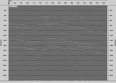
Figure 11. Vertical component final stacking , (P wave), Line EW

Processing of this line mainly follows the same steps as line A processing. However, these data are affected by a larger geological complexity, which renders the application of the methods applied there less effective. Particularly, the image of a reflector guiding the statics correction iterations is more uncertain.

Figure 13. Effect of the relative source – receiver direction and PS converted wave dip

Differences between positive and negative offsets images are also apparent, as it is shown in Figures 12a and 12b. The events correspond to different points within the subsoil. Furthermore, there is a different velocity field for each type of offset. For instance, comparing the event which appears at 900 ms, which seems closer to CDP 760 for positive offsets, and to CDP 800 for negative offsets, the stacking velocity is around 150 m/s larger for negative offsets.

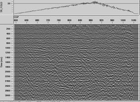
Figure 12(a). Line B: positive offset stacking

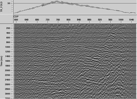
Figure 12(b). Line B: negative offset stacking

An explanation to this phenomenon can be found in the difference in PS wave times (that is to say, processing velocities), according to direction (Thomsen, 1999). The explanation is based upon the path asymmetry or presence of heterogeneity, as it is illustrated in Figure 12, which does not occur in P waves. Since there is asymmetry in the field properties (represented in this case by the reflector dip), the times and velocities are different. In Figure 12, we assume both raypaths to have the same source - receiver distance, but Vc velocity is smaller in the positive offset (left to right), since it has a larger percentage of the trajectory as S wave. This PS wave asymmetry makes it necessary to resort to more advanced processing methods.

Fracture analysis with converted waves

A true relative amplitude, surface-consistent processing flow was used to ensure that the input data satisfy the requirements of the birefringence analysis algorithm. The final stacked sections of the radial and transverse components, which have been processed in a fully surface-consistent fashion so that they can be properly analyzed for birefringence, are shown in Figure 14.

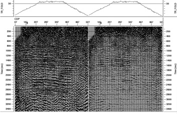
Figure 14. Final true relative-amplitude, surface-consistent stacks of the radial component (left) and the transverse component (right) of NL-99-983

There are a number of observations that we can make about these two stacks. First, we see that there is coherent energy present on both stacks, although there is obviously much more energy on the radial stack than on the transverse stack. The fact that there is coherent reflection energy on the transverse stack is an indication that shear-wave splitting is likely occurring here. However, other effects such as cross-dipping geology or misoriented geophones can also put energy on the transverse component. Notice that several of the wavelets on the events on the transverse stack appear to be about 90 degrees out of phase with the events on the radial stack (peaks correspond to zero-crossings, and vice versa). This 90 degree phase difference is expected when a single anisotropic layer is causing shear-wave splitting (Cary, 2002). This observation makes it more plausible that the energy on the transverse component is caused by shear-wave splitting. Random errors in the orientation of geophones would tend to stack out. Consistent energy on the transverse component would only occur if there is a consistent error in geophone orientation, and we assume that this did not occur during acquisition.

The events on the radial stack are much higher in amplitude than the comparable events on the transverse stack. This is to be expected when there is shear-wave splitting present, and the direction of the 3C seismic line is fairly close to the direction of either the fast (S1) direction or the slow (S2) direction associated with the so-called “natural” coordinate system associated with the fracturing. The only situation in which you would expect equal amounts of energy on both the radial and transverse stacks is when the natural coordinate system is at a 45 degree angle to the seismic line. At all other angles, there should be more energy on the radial component than on the transverse component (Winterstein, 1992).

Notice that the coherent events on the transverse component stack occur mainly within the high-fold portion of the stack, where the suppression of noise from stacking is most strong. This might indicate that the splitting actually occurs over a wider area than is indicated by the events on the transverse stack, but that the signal-to-noise level outside the central portion of the stack is simply too low to indicate it.

Notice that the coherent events on the transverse stack extend almost vertically from deep in the section to the shallow section. This is an indication that the shear wave splitting starts to occur in a shallow part of the seismic section. Suppose that shear-wave splitting were occuring only at 2,5 seconds, and no where else in the section. Then reflection events would be visible on the transverse section below 2,5 seconds, but not above 2,5 seconds. So the fact that reflection events occur throughout the transverse stack indicates that the splitting must start in the shallow part of the section.

If splitting were occuring deep in the section as well as in the shallow section, then we should be able to see a difference either in the direction of S1 or in the time delay between the S1 and S2 wavefields. Figure 15 shows three sets of time gates that were used for birefringence analysis. Figure 16 shows the result of birefringence analysis within the shallow gate, and just for CDP's 263 to 349 in the middle of the stack. Notice that the maximum time delay in this plot is 100 ms, which is very large. A 100 ms time delay would mean that the S1 arrival is a full 100 ms before the S2 arrival.

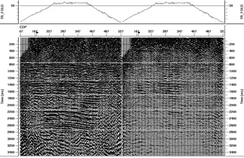
Figure 15. The top pair of green lines indicates the first birefringence analysis gate, the middle pair of lines indicate the second analysis gate, and the bottom pair of lines indicate the third analysis gate. The bottom pair of lines encloses the zone of interest (La Luna-Tiba Formation)

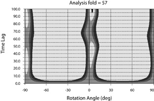
Figure 16. Results of the birefringence analysis within the shallow analysis gate for CDP's 293 to 349 for time delays between S1 and S2 arrivals of up to 100 ms. Notice that there are four separate maxima, but that the top two maxima in the Figure are “repeats” of the bottom two caused by the oscillatory nature of the data. The period is about 60ms, which is the dominant frequency of the data. Therefore only time delays up to 60 ms are shown in later plots

There are four separate maxima within the contour plot in Figure 16 but they repeat themselves (along lines of equal azimuth) after the first 50 to 60 ms. This is because the crosscorrelation function has a periodicity that is the same as the dominant period of the wavelet in the data, which is about 60 ms. The contoured maximum with the highest peak value indicates that the time lag and azimuth at the maximum is able to match the data the best. In this case there are large maxima at about 44 ms and at about 100 ms. Although there is no absolute way of knowing which of these is the right one, we assume that the smaller time lag (44 ms) is far more likely to occur. Secondary maxima, such as the peaks along the –86 degree azimuth line, always occur because of the oscillatory nature of the cross-correlation function.

Figures 17, 18 and 19 show the results of the birefringence analysis within the shallow, middle and deep portions of the stacks for the same traces (CDP's 293 to 349). There is little difference in the direction of S1, or in the time delay between S1 and S2 for the shallow section (4° and 44 ms) and the middle layers (10° and 44 ms). This implies that the shear-wave splitting is likely occurring in the shallowest part of the section, above the top analysis gate, but not within the middle layers. It is questionable whether the difference between 4° and 10° in the shallow and middle layers is significant since the data processing is probably not accurate enough to believe that such small differences are significant.

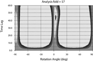
Figure 17. The strongest peak of the birefringence analysis within the top analysis gate (CDP's 293 to 349) indicates that the fast (S1) direction is at an angle of 4 degrees (clockwise) with respect to the line direction, and that the time delay between S1 and S2 is 44ms. The secondary peak at an angle of –86 degrees does not generate as good a fit to the data so it is not considered to be the correct result

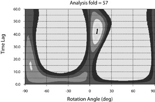
Figure 18. Results of the birefringence analysis within the middle analysis gate (CDP's 293 to 349) indicate that the fast (S1) direction is at an angle of 10 degrees (clockwise) with respect to the line direction, and that the time delay between S1 and S2 is 44 ms. This result is very similar to the result for the top layer, which indicates that there is little effect of splitting within the middle part of the section

Figure 19 shows the birefringence analysis for the bottom gate which indicates that the azimuth stays much the same as for shallower layers (4°), but that the time delay is reduced to 28 ms. Theoretically, a reduction in time delay is not easily explained without a change in the azimuth of the fractures, so what is probably happening to cause this result is that the azimuth angle actually changes within the La Luna Formation. In order to get a more accurate estimate of the birefringence within the La Luna Formation, the effects of the shallow birefringent layers need to be stripped off.

Figure 19. Results of the birefringence analysis within the bottom analysis gate (CDP's 293 to 349) indicate that the fast (S1) direction is at an angle of 4 degrees (clockwise) with respect to the line direction, and that the time delay between S1 and S2 is 28 ms

The effect of the upper layer birefringence is to rotate 10° from radial/transverse to S1/S2 coordinates, time delay S2 by 44 ms, and then rotate -10° from S1/S2 coordinates to radial/transverse acquisition coordinates. To strip off these effects, we do the reverse: rotate 10° from radial/transverse to S1/S2 coordinates, time advance S2 by 44 ms, and rotate -10° to get back to radial/transverse coordinates.

Figure 20 shows the result of rotating the radial and transverse stacks 10° clockwise into the S1 and S2 coordinate system as indicated by the analysis of the middle layers of the stack. In many studies, the data have been analyzed in this dominant coordinate system. For example, Mueller (1992) provides evidence that amplitude dimming on the S2 stack is indicative of an increase in fracturing within the Austin Chalk formation in Texas.

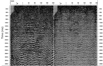
Figure 20. S1 stack (left) and S2 stack (right) generated by rotating the radial and transverse stacks 10 degrees clockwise into the natural coordinate direction indicated by analysis of the middle layer. According to Mueller (1992, The Leading Edge), the weak amplitudes on the S2 stack within the zone of interest can be interpreted as zones of increased fracturing

Figure 21 shows the result of stripping off the layers above the La Luna Formation in the manner previously described. Ideally, the effect of doing this would be to put all the reflection energy above the bottom reflector onto the radial component stack. Obviously this has not happened, although some reduction in the energy on the transverse stack is visible. Presumably the major reason for this imperfect result is that the birefringence analysis has yielded only average results over the analysis gate. Lateral variations could account for the differences. It appears that in areas outside the central part of the stacks, additional energy has leaked onto the transverse stack from the radial component due to this lateral variation factor. An additional factor could certainly be that the high level of noise in the data has made a completely accurate surface-consistent processing flow impossible.

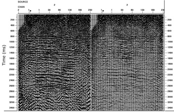
Figure 21. Radial (left) and transverse (right) stack after stripping off the middle layer above the zone of interest. Stripping off the middle layer involved rotating 10 degrees from radial/transverse to S1/S2 coordinates, removing the time delay of 44 ms from the S2 component, and rotating –10 degrees back to the radial/transverse coordinates. The fact that energy remains on the transverse component in the middle layer probably indicates that lateral variations in shear-wave splitting have not been removed from the data

Finally, Figure 22 shows the result of birefringence analysis within the zone of interest of the stacks in Figure 21. The indication is that the direction of splitting within La Luna is slightly counterclockwise (by about 5°) with respect to the seismic line direction, and the average time delay within CDP's 293 to 349 is about 32 ms.

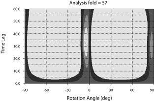
Figure 22. Birefringence analysis within the zone of interest (CDP's 293 – 349) after the layer above it has been stripped off. The maximum occurs at –5 degrees, with a time delay of 32 ms

CONCLUSIONS

• For line A a polarization anomally was detected in the converted waves, which could be interpreted as being caused by the presence of a fracture train. Nevertheless this is not conclusive, since there could exist other anisotropy causes aside from fractures (e.g. pressures).

• The seismic processing methods considering polar anisotropy (VTI) showed to be effective in the process of obtaining information from the converted wave data from multi—component lines shown here.

• It is remarked that two types of anisotropy were dealt independently with along this work, VTI anisotropy for processing, and HTI anisotropy for fracture analysis, however with meaningful results. A more accurate method would integrate these two approaches.

• A strong reflector is observed in the converted wave section, which arrives at an approximate 1000 ms time on line A (NS). This reflector was interpreted as the interface joining the base of Carbonera formation, mainly shale coal and sandstone, with the top of Mirador Formation, mainly sandstone. It shows lithological meaning on converted wave data, since from the literature (e. g. Tatham and McCormack, 1991) the interface shale-sandstone typically has higher impedance for S waves than for P-waves. However data from boreholes could support or deny this hypothesis.

• A main difficulty in converted wave data processing was correction of receiver statics. An effective result was obtained with the method used to obtain such correction here, based upon the common receiver stacks. One difficulty with this method is that a circular relationship is generated between the receiver statics correction and the stacking velocity analysis, since common receiver stacks depend on the velocities, which require a good statics correction themselves. The study of weathering layer characteristics and its effect on S-wave deserves more effort, in order to improve the statics correction on the receiver for converted waves. The method used on line A appeared effective, however appears not as successful for more complicate settings (as Line B).

• The dip line poses larger difficulty, mainly due to its structural complexity. Theories have been proposed (e. g. Thomsen, 1999; Herrenschmidt et al ., 2001), which take into consideration specific characteristics of this type of data, such as beam trajectory asymmetry, the effect of anisotropy on horizontal layers, etc. and methods such as tomography and pre- stack depth migration. However complex areas in land are yet challenging for converted wave processing methods.

• The conclusions of this study of Line A are that the data appears to indicate the existence of at least two birefringent layers, one in the shallow section which is 4° to 10° clockwise with respect to the seismic line direction, and one within the La Luna Formation which is about 5° counter clockwise with respect to the line direction. The estimated time delays between S1 and S2 arrivals are relatively large (44 ms and 32 ms respectively). It is assumed that the 3C geophones use a right handed coordinate system to obtain this result.

• It is strongly recommended that the results of this study not be trusted on their own. Complementary borehole information and processing of the other seismic lines would give a strong support to any final conclusion. Ideally all three lines would yield consistent results from birefringence analysis, which would generate a lot more confidence in the results than the analysis of this single line by itself.

• The complete interpretation of the birefringence analysis should include the meaning of the delay time and the anisotropy angle. Theories proposed, (e. g. Hudson, 1981) would allow to infere fracture density from this information. It would be a valuable future development to apply these theories and compare their result with well test information, to obtain information about azimuthal anisotropy on the line, to confirm if that anisotropy is caused by fractures or other event, and if it is caused by fractures, to obtain a fracture model of this area.

ACKNOWLEDGEMENTS

REFERENCES

Aguilera, R. (1998). Geologic aspects of naturally fractured reservoirs. Leading Edge, 17: 1667-1670.         [ Links ]

Alford, R. M. (1986). Shear data in the presence of azimuthal anisotropy: Dilley, Texas. 56th Annual International Meeting. SEG Expanded Abstracts, 476-479.         [ Links ]

Anno, P. D. (1986). Two critical aspects of shear-wave analysis: statics solutions and reflection correlations. In Shear-wave exploration. (S.H. Danbom and S. N. Domenico Eds.), SEG Geophysical development series. 1. Tulsa.         [ Links ]

Ata, E., & Michelena, R. (1995). Mapping distribution of fractures in a reservoir with P-S converted waves. Leading Edge, 14: 664-676.         [ Links ]

Cary, P. (2002). Detecting false indications of shear-wave splitting. 72nd Annual International Meeting, SEG. Expanded Abstracts, 1014-1017.         [ Links ]

Cary, P. W., & Eaton, D. W. S. (1993). A simple method for resolving large converted wave (P-SV) statics. Geophysics, 58: 429-433.         [ Links ]

Crampin, S. (1985). Evaluation of anisotropy by shear-wave splitting. Geophysics, 50 (1), 142-152.         [ Links ]

Garotta, R. (2000). Shear-waves from acquisition to interpretation. SEG Distinguished Instructor Series, 3.         [ Links ]

Harrison, Mark. (1992). Processing of P-SV seismic data: anisotropy analysis, dip move-out and migration. Tesis Ph. D. Universidad de Calgary, Canada.         [ Links ]

Herrenschmidt, A., Granger, P. Y, Audebert, F., Gerea, C., Etienne, G., Stopin, A., Alerin, M., Lebegat, S., Lambare, G., Berthet, P., Nebieridze, S., & Boelle, J. L., (2001). Comparison of different strategies for velocity model building and imaging of PP and PS real data. Leading Edge, 984-995.         [ Links ]

Hudson, J. A. (1981). Wave speeds and attenuation of elastic waves in material containing cracks. Geophys. J. R. Astron. Soc. 64:133-150.         [ Links ]

Mueller, M. C. (1992). Using shear waves to predict lateral variability in vertical fracture intensity. Leading Edge, 11: 29-35.         [ Links ]

Rüger, A. & Tsvankin, I. (1997). Using AVO for fracture detection: analytic basis and practical solutions. Leading Edge, 16: 1429-1434.         [ Links ]

Stewart, R. R., Gaiser, J., Brown, R. J., & Lawton, D.C., (2002). Converted-wave seismic exploration: Methods. Geophysics, 67 (5), 1348-1363.         [ Links ]

Tatham, R. H. & McCormack, M. D. (1991). Multicomponent seismology in Petroleum Exploration. SEG Investigations in Geophysics.         [ Links ]

Thomsen, L. (1999). Converted-wave reflection seismology over inhomogeneous, anisotropic media. Geophysics, 84 (3), 678-690, May-Jun.         [ Links ]

Thomsen, L. (2002). Understanding seismic anisotropy in exploration and exploitation. SEG-EAGE Distinguished Instructor Series, 5.         [ Links ]

Villamil, Tomás. (2001). La búsqueda de petróleo bajo La Luna. Carta Petrolera, Edición especial de Aniversario.         [ Links ]

Winterstein, D. (1992). How shear-wave properties relate to rock fractures: simple cases. Leading Edge, 21-28, Sept.         [ Links ]

Wiggins, R., Larner, K., & Wisecup, R., (1976). Residual statics as a general linear inverse probem. Geophysics, 41 (5), 922-938, Oct.         [ Links ]

Yilmaz, O. (1987). Seismic data processing. SEG Investigations in Geophysics, Tulsa.         [ Links ]