ABSTRACT

In this study pressure test analysis in wells flowing under constant wellbore flowing pressure for homogeneous and naturally fractured gas reservoir using the TDS technique is introduced. Although, constant rate production is assumed in the development of the conventional well test analysis methods, constant pressure production conditions are sometimes used in the oil and gas industry. The constant pressure technique or rate transient analysis is more popular reckoned as "decline curve analysis" under which rate is allows to decline instead of wellbore pressure.

The TDS technique, everyday more used even in the most recognized software packages although without using its trade brand name, uses the log-log plot to analyze pressure and pressure derivative test data to identify unique features from which exact analytical expression are derived to easily estimate reservoir and well parameters. For this case, the "fingerprint" characteristics from the log-log plot of the reciprocal rate and reciprocal rate derivative were employed to obtain the analytical expressions used for the interpretation analysis. Many simulation experiments demonstrate the accuracy of the new method. Synthetic examples are shown to verify the effectiveness of the proposed methodology.

Key words: radial flow, closed system, pseudosteady state, interporosity flow parameter, dimensionless storage coefficient, fracture dominated period, transition period.

RESUMEN

En este estudio se introduce el análisis de pruebas de presión en pozos de gas que fluyen a presión de fondo constante en formaciones homogéneas y naturalmente fracturadas usando la técnica TDS. Aunque normalmente se considera la producción de un pozo a caudal constante en el desarrollo de los métodos convencionales de interpretación de pruebas de pozos, el caso de producción de un pozo a condiciones de presión constante se usa en algunas ocasiones en la industria de los hidrocarburos. La técnica de presión constante o análisis de transientes de caudal se conoce más popularmente como "análisis de curvas de declinación" en la cual se permite que la rata de flujo decline en vez de hacerlo la presión del pozo.

La técnica TDS se vuelve más popular cada día incluso en la mayoría de los programas comerciales que aunque sin usar su nombre de pila, usan el gráfico log-log para analizar datos de presión y la derivada de presión para identificar características únicas de las cuales se derivan relaciones analíticas exactas para estimar fácilmente los parámetros del yacimiento y el pozo. Para este caso "las huellas digitales" características procedentes del gráfico log-log del recíproco del caudal y la derivada del recíproco del caudal se emplearon para obtener expresiones analíticas que se usan para propósitos de interpretación. Se usaron muchas corridas de simulación para demostrar la exactitud del nuevo método. Se muestran ejemplos sintéticos para verificar la efectividad de la metodología propuesta.

Palabras Clave: flujo radial, sistema cerrado, estado pseudoestable, parámetro de flujo interporoso, coeficiente de almacenamiento adimensional, periodo dominado por las fracturas, periodo de transición.

INTRODUCTION

Normally, well test interpretation methods assume well production at a given constant rate. However, several common reservoir production conditions result in flow at a constant pressure, instead. Such is the case in wells producing from low permeability formations which often become necessary the production at a constant wellbore flowing pressure.

A gas or oil well producing at constant bottomhole pressure behaves analogously to that of a well operating at constant flow rate. In a constant pressure flow testing, the well produces at a constant sandface pressure and flow rate is recorded with time. Since rate solutions are found on basic flow principles, initially solved by Van Everdingen and Hurst (1949), flow rate data can be used for reservoir characterization. Therefore, this technique becomes in an alternative to conventional constant flow rate well testing techniques.

Several rate analysis methods are presented in the literature. The most popular method is the decline curve analysis presented by Fetkovich (1980) which is only applicable to circular homogeneous reservoirs. This technique assumes circular homogeneous reservoir and is not applicable to heterogeneous systems. The main drawback of type-curve matching, used by Fetkovich, is basically the involvement of a trial and error procedure which frequently provides multiple solutions. Therefore, a procedure used by Tiab (1995), TDS technique, avoids using type-curve matching since particular solutions are obtained from the pressure and pressure derivative plot providing a very practical methodology for interpretation of well tests. The application of the TDS technique to constant bottomhole pressure tests is not new. It was first introduced by Arab (2003) for the case of oil in homogeneous and heterogeneous reservoirs. Then, in this work, we extend Arab's work for gas well test interpretation.

MATHEMATICAL MODELING

Homogeneous reservoirs

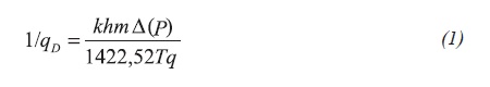
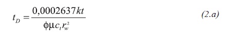
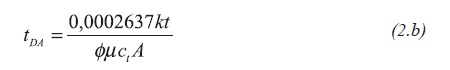
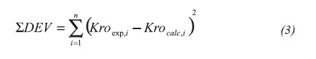
The dimensionless quantities are defined as follows in Equations 1, 2.a, 2.b, and 3:

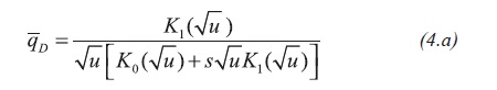
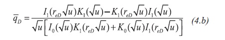
The solutions to the flow equation under constant well pressure for an infinite reservoir including wellbore damage, Van Everdingen and Hurst (1949), and bounded reservoir, DPrat, Cinco-Ley, and Ramey (1981), respectively, are Equations 4.a and 4.b:

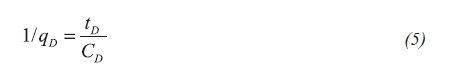
By analogy with transient pressure analysis, during the early time period of the reciprocal rate a unit-slope line is identified. The equation of this line is Equation 5:

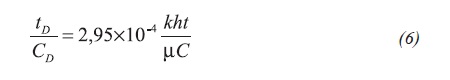
The relationship t_D/C_D is obtained from the combination of Equations 2.a and 3:

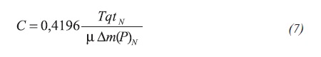
Substituting Equations 1 and 6 into Equation 5 will result an expression for the wellbore storage coefficient:

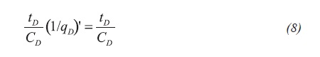
The reciprocal rate derivative also has a unit-slope line at early times. Its equation is Equation 8:

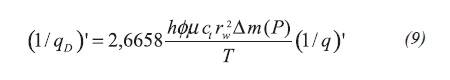
The derivative of the reciprocal flow rate is given by:

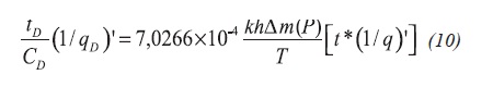
The left-hand side of Equation 8 can be combined by replacing Equations 6 and 9 and after multiplying and diving by 0,8935 (to replace by C_D) and taking C_D as 1, finally results in Equation 10:

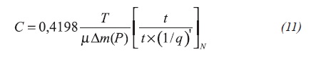
Also, during the early time period the reciprocal rate derivative has a unit-slope line is identified, which allows to obtain Equation 11:

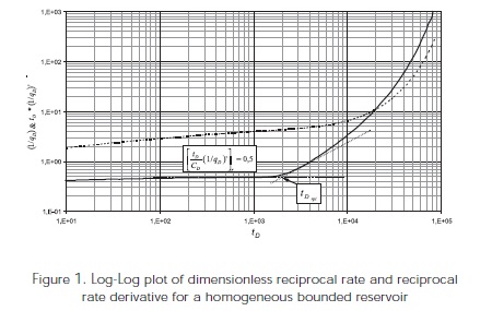
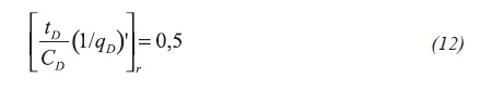
As shown in Figure 1, the horizontal line of the reciprocal pressure derivative during infinite- acting behavior is described by Equation 12:

Combining Equations 10 and 12 results in an expression to estimate formation permeability,

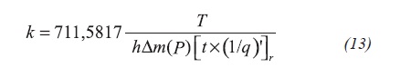
According to Tiab (1995) the starting time of the infinite-acting line of the reciprocal rate derivative can be approximated by Equation 14:

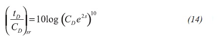
Plugging Equation 6 and 3 into Equation 13 provides an equation to estimate the starting time of the radial flow regime:

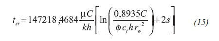
According to Vongvuthipornchai and Raghavan (1988), the start of the radial flow line is represented by Equation 16:

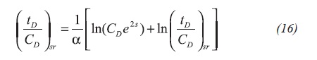
Being α a tolerance factor which may be substituted by 0,05 giving results within 8% of accuracy. Replacing Equation 3 into Equation 16, it yields in Equation 17:

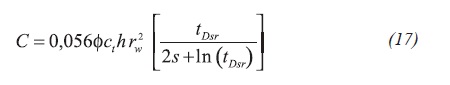
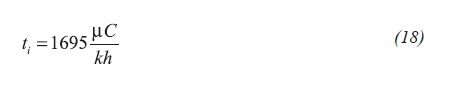
t_Dsr is found from Equation 2.a for t = t_Dsr. From the intercept between the early unit-slope and radial lines results in an expression useful to verify permeability, Equation 18:

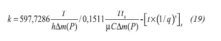
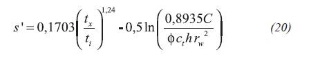
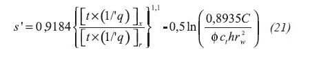
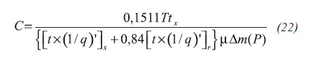
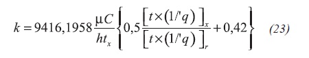
Tiab (1995) correlated permeability, skin factor and wellbore storage coefficient with the maximum pressure derivative point during the early transition period. By analogy, from those correlations we obtain Equations 19, 20,21, 22 and 23:

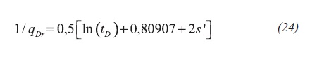
For constant pressure production during radial, t_D > 8000, the reciprocal rate behavior including skin factor obeys the following behavior, Equation 24:

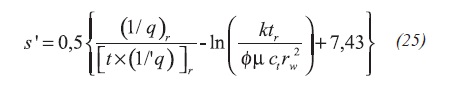
Dividing Equation 24 by Equation 12, plugging the dimensionless quantities and, then, solving for the apparent skin factor results Equation 25:

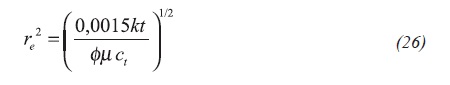
Arab (2003) found that the pseudosteady state develops when t_DA = 0,0054 (t_DApss = 0,0054). Replacing this into Equation 2.b and knowing that for circular systems A = πr_e², the external radius can be found as Equation 26:

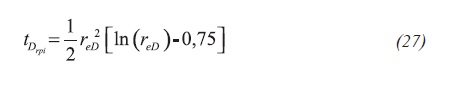
As seen in Figure 1, the intercept formed between radial and pseudosteady state lines of the dimensionless reciprocal derivative is defined as, Arab (2003):

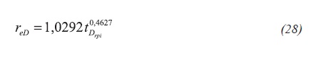
Which numerical solution, Arab (2003), leads to Equation 28:

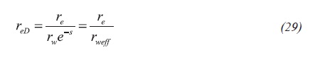
Defining the dimensionless external radius by Equation 29:

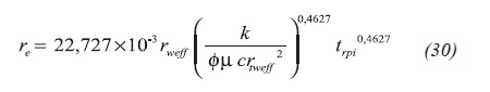
After replacing Equation 2.a and 29 into Equation 28 yields in Equation 30:

Heterogeneous reservoirs

Transition period occurs during radial flow regime

Redefining Equation 2.b:

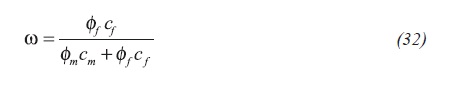
From here on, k in Equation 1 and 3 is replaced by k_ƒ representing the network fracture permeability. The naturally fractured reservoir parameters, Warren and Root (1963), are given by Equation 32:

Here α means "proportional" and is not the same as in Equation 16. Define the reservoir storativity as Equation 34:

The solution of the diffusivity equation for an infinite and bounded heterogeneous reservoir, respectively, was presented by DPrat, Cinco-Ley, and Ramey (1981):

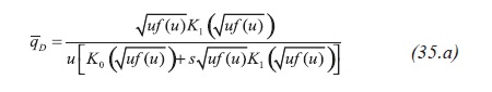
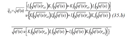
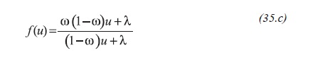
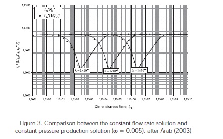
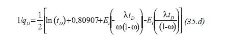
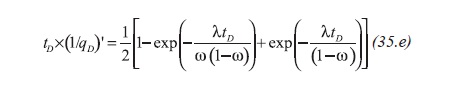
Arab (2003) found that the solution for the pressure and reciprocal rate behaves similarly, Figure 3, then, the reciprocal rate solution and its derivative for a naturally fractured reservoir obey the following expressions, Equations 35.d and 35.e :

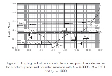
In Figure 2, it is observed that the radial flow period has two segments. The first corresponds to fluid depletion inside the fracture network and the second one is the answer of a homogeneous system. Then, as for the homogeneous case, the pressure derivative during this period is represented by an expression similar to Equation 12:

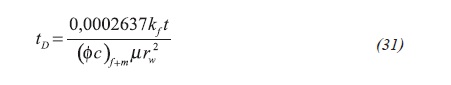
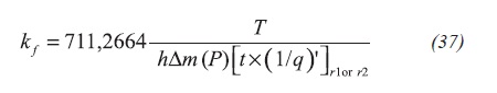
Again, after plugging the dimensionless quantities as for the homogeneous case, taking care that the dimensionless time is now represented by Equation 31, will result Equation 37:

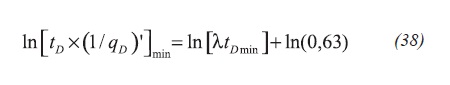
Similarly to the procedure achieved by Engler and Tiab (1996), a log-log plot [t_D*(1/q_D)']_min vs. (λt_D)_min results in a unit-slope straight line which equation is given by Equation 38:

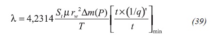
After replacing the dimensionless expressions and solving for the interporosity flow parameter,

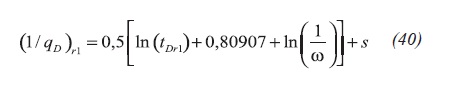
The transient behavior of a double porosity formation during the fracture-dominated period is given by, Engler and Tiab (1996), Equation 40:

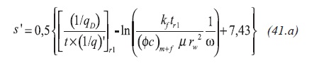
After dividing the above relationship by Equation 36, replacing the dimensionless parameters and solving for the apparent skin factor results Equation 41.a:

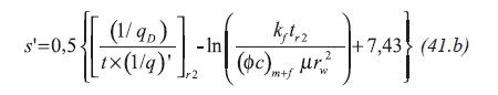
Once the transition period vanishes, the system behaves as homogeneous, then ω = 1, and Equation 41.a becomes Equation Equation 41.b:

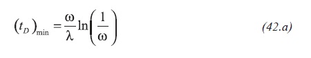
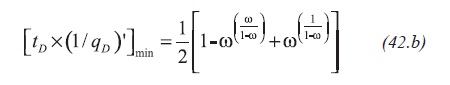
Referring to Figure 2, as expressed by Engler and Tiab (1996), the minimum point coordinates of the reciprocal rate derivative are Equations 42.a and 42.b:

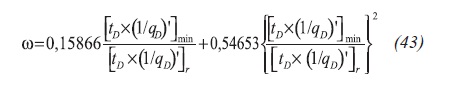
Engler and Tiab (1996) divided Equation 42.b by Equation 36 and plotted the ratio of the minimum and the radial pressure derivatives against the dimensionless storativity ratio. By the analogy obtained from Figure 3, the expression their expression is formulated as Equation 43:

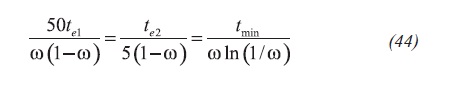
Following the work done by Engler and Tiab (1996) and later by Arab (2003), the following relationship is presented in Equation 44:

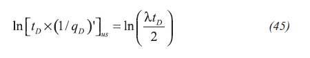
Arab (2003) defined the unit-slope line during the transition period as Equation 45:

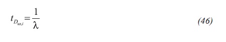
From the intercept point formed by the radial flow and the unit-slope lines will result Equation 46:

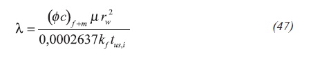
Plugging Equation 31 into the above expression yields in Equation 47:

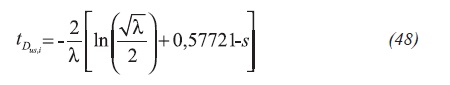
Equation 45 can be written as Equation 48:

Also, replacing Equation 31 in the former equation results Equation 49.a:

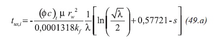
Equation 49.a is useful to verify the value of λ. Other equations used in the conventional method to find the naturally fractured reservoir parameters can be applied for the case of constant pressure case, i.e., the equation presented by Tiab and Escobar (2003).

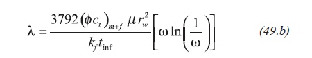
Being tinf the inflection point found during the transition period on the semilog plot. This time value also corresponds to the minimum point of time, t_min, found on the pressure derivative plot. Therefore, Equation 49.b forms part of the TDS technique.

Transition period occurs during late-pseudosteady state flow regime

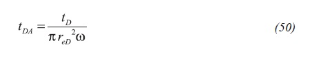
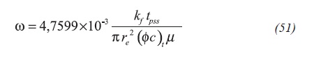
The dimensionless time based upon area for a heterogeneous formation can be expressed by Equation 50:

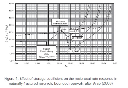
As seen in Figure 4, Arab (2003) found that the pseudosteady state develops when t_DApss = 0,00554. Assuming that the skin factor is zero in Equation 29, then from Equation 50 will result Equation 51:

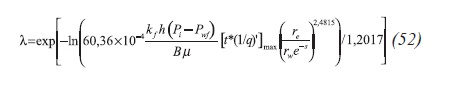
Arab (2003) found the following correlation using the maximum point on the pressure derivative curve when the transition period initiates. Equation 52:

Figures 4 and 5 show the different features found on the plot of reciprocal rate and reciprocal rate derivative. The unit-slope line of the transition period during the pseudosteady state, Figures 4 and 5, is governed by, Arab (2003):

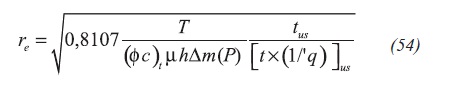
Replacing the dimensionless equations an expression to obtain drainage area from any arbitrary point during the pseudosteady-state line (transition period) is obtained Equation 54:

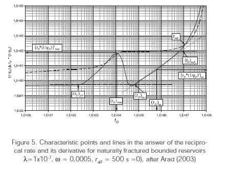
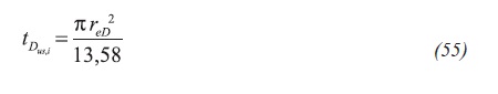
The intersection between the unit-slope and the radial flow lines, Figure 5, provides Equation 55:

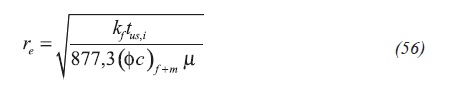
A new expression to obtain the drainage area will result after replacing the respective dimensionless quantities, Equation 56:

Combination of Equation 51 and 56 will give,

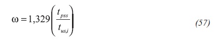
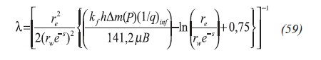
The dimensionless reciprocal rate curve presents a horizontal or constant behavior during the matrixfracture transition period, Figure 5, which allows to obtain λ, Equation 58:

As before, the following equality is found after replacing the dimensionless expressions, Equation 59:

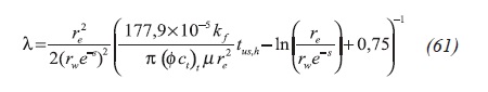
The intersection of the unit-slope line during the transition period and the characteristic horizontal line of the reciprocal rate curve, also during the transition period, provides an expression which leads to calculate λ, see Figure 5:

After plugging the dimensionless quantities, as before, yields in Equation 61:

An especial feature of the reciprocal rate curve is that it intercepts with the reciprocal rate derivative providing the following governing Equation 62:

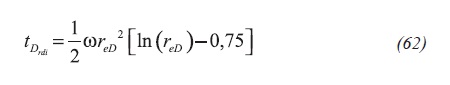
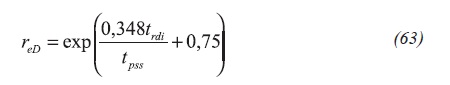
Suffix "rdi" stands for the intersection of the reciprocal rate curve and the reciprocal rate curve derivative. Combining this with Equation 50 will yield in Equation 63:

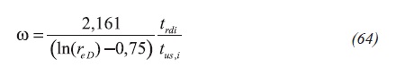
Also, combination of Equation 55 and 62 will result in Equation 64:

TOTAL SKIN FACTOR

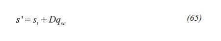
The apparent skin factor is defined by Equation 65:

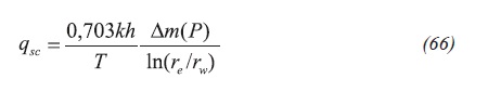
Many flow rates take place for the constant bottomhole pressure case. Then, assuming steady-state Darcy's flow applies Equation 66:

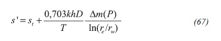
Then, using Equation 66, Equation 65 can be written as:

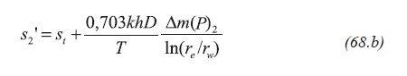
It is suggested to run two well tests at different bottomhole pressure values so a procedure similar to the one outlined by Nuñez-Garcia, Tiab and Escobar (2003) can be applied for obtaining the total skin factor. Then Equation 68.a,

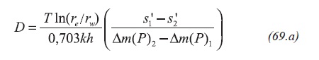
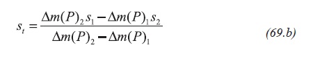
The simultaneous solution of Equation 68.a and 68.b leads to obtain D and S_t values,

EXAMPLES

Example 1

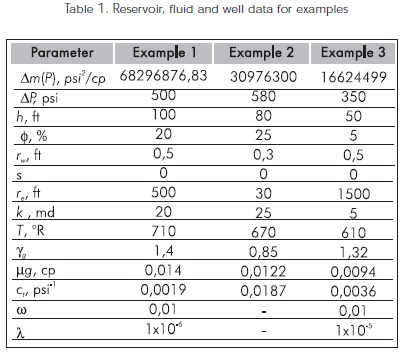
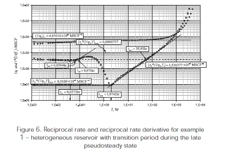
The reciprocal rate and reciprocal rate derivative for a simulated well test of a naturally fractured reservoir with the transition period taking place during the late pseudosteady-state flow is shown in Figure 6. The input data for the simulation is given in Table 1. Find reservoir permeability, skin factor, drainage radius, interporosity flow parameter and dimensionless storativity coefficient for this problem.

Solution

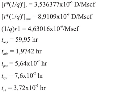
The following characteristic points are read from Figure 6.

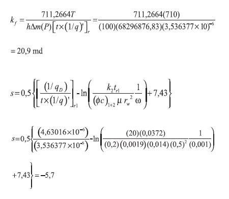
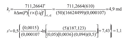
Permeability and apparent skin factor are obtained from Equation 37 and Equation 41.a, respectively,

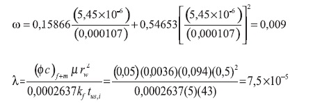
The dimensionless storativity coefficient and interporosity flow parameter are respectively estimated from Equation 43 and 47.

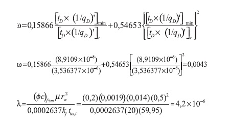
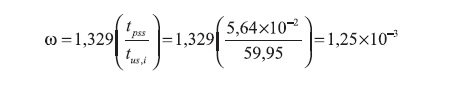
Again, the dimensionless storativity coefficient is estimated using Equation 57, thus:

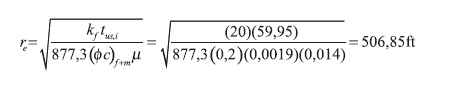
The drainage radius is estimated with Equation 56,

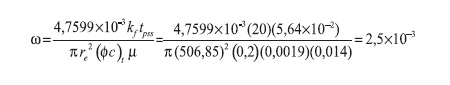
Once again, the dimensionless storativity coefficient is recalculated with Equation 51, thus:

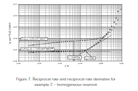
Example 2

Figure 7. presents the reciprocal rate and reciprocal rate derivative for a simulated well test of a homogeneous bounded reservoir. As for example 1, the data used for the simulation is given in Table 1. Find reservoir permeability, skin factor and drainage radius for this example.

Solution

The following information is read from Figure 7:

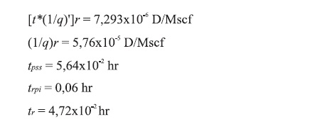
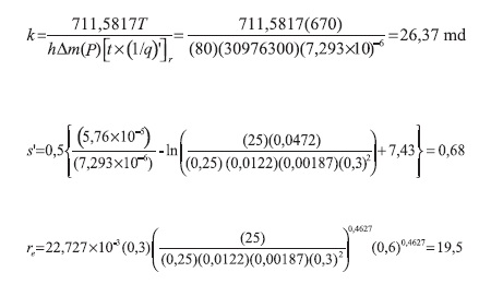
Equations. 13, 25 and 30, are used to obtain permeability, skin factor and drainage.

Example 3

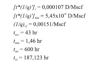
The reciprocal rate and reciprocal rate derivative for a simulated well test for a naturally fractured reservoir with the transition period taking place during the radial flow regime is shown in Figure 8. The input data for the simulation is also given in Table 1. For this example find reservoir permeability, skin factor, drainage radius, interporosity flow parameter and dimensionless storativity coefficient.

Solution

The following characteristic points are read from Figure 6.

Permeability and apparent skin factor are obtained from Equations 37 and 41.b, respectively,

The naturally fractured reservoir parameters are estimated with Equations 43 and 47,

ANALYSIS OF RESULTS

From the simulated examples is observed that the estimated parameters are in good agreement with the input values, except for the apparent skin factor which presents some variations from simulated runs in fractured wells and naturally fractured reservoirs. However, based upon the good results, there is implied that the TDS technique works accurately and practically. For space saving purposes not all the equations were reported in the worked examples. However, they also present a good degree of accuracy and may be applied by the reader in his/her own field of practice. Finally, the differences between the simulated and estimated skin factors may be due to turbulence effects.

CONCLUSIONS

• For multiphase flow, new equations are introduced to the TDS technique for estimation of phase permeabilities, wellbore storage coefficient, skin factor and reservoir drainage area. The application of the equations was verified through field and simulated well test data.

• A new set of equations for interpretation of well test data from constant bottomhole pressure is presented following the philosophy of the TDS technique. These equations were proved to work accurately with synthetic test data.

• The results provided in this article show that well test analysis methods for wells produced at constant pressure provide the same information about the reservoir as is determined from the conventional methods for the constant-rate production case. Therefore, the transient rate data analysis may be used as an alternative method in the absence of the transient pressure data.

• Unlike the typical decline-type curves presented by Fetkovich, the results obtained by the TDS technique are verifiable. The solutions provided here reveal that the various sorts of reservoir heterogeneities affect the rate behavior which is reflected when having the transition period during the late pseudosteady state period and, due to due to the rate exponential behavior, the reciprocal rate and pressure solutions are very different for boundary dominated flow period. Therefore, the decline-type curves may not be able to capture these details and may lead to unreliable results.

ACKNOWLEDGMENTS

The authors gratefully acknowledge the financial support of both Ecopetrol S.A.-Instituto Colombiano del Petróleo (ICP) and Universidad Surcolombiana, Neiva, Huila.

REFERENCES

Arab, N. (2003). Application of Tiab's Direct Synthesis Technique to Constant Bottom Hole Pressure Tests. M. S. Thesis, The University of Oklahoma, USA.        [ Links ]

DaPrat, G., Cinco-Ley, H., & Ramey, H. J. Jr. (1981). Decline Curve Analysis Using Type Curves for Two-Porosity System, June. SPEJ 354-62.        [ Links ]

Engler, T. and Tiab, D., (1996). Analysis of Pressure and Pressure Derivative Without Type Curve Matching, 4. for Naturally Fractured Reservoirs. J. Petroleum Scien. and Engineer., 15:127-138.        [ Links ]

Fetkovich, M. J. (1980). Decline Curve Analysis Using Type Curves. J. Petroleum Technol., June, 1065-1077.        [ Links ]

Nuñez-García, W., Tiab, D., & Escobar, F. H. (2003). Transient Pressure Analysis for a Vertical Gas Well Intersected by a Finite-Conductivity Fracture. SPE Production and Operations Symposium, Oklahoma City, OK, U.S.A., March 23–25. SPE 15229.        [ Links ]

Tiab, D. (1995). Analysis of Pressure and Pressure Derivative without Type-Curve Matching: 1- Skin Factor and Wellbore Storage. J. Petroleum Scien. and Engineer., 12: 171-181.        [ Links ]

Tiab, D. & Escobar, F. H. (2003). Determinación del Parámetro de Flujo Interporoso a Partir de un Gráfico Semilogarítmico. X Congreso Colombiano del Petróleo., Bogotá, Colombia, Oct. 14-17.        [ Links ]

Van Everdingen, A. F., & Hurst, W. (1949). The Application of the Laplace Transformation to Flow Problems in Reservoirs. Trans. AIME (Amer. Inst. Min. Metall. Eng.), 186: 305-320.        [ Links ]

Vongvuthipornchai, S., & Raghavan, R. (1988). A Note on the Duration of the Transitional Period of Responses Infl uenced by Wellbore Storage and Skin. SPE Formation Evaluation, 207-214.        [ Links ]

Warren, J. E. & Root, P. J. (1963). The Behavior of Naturally Fractured Reservoir. Soc. Pet. Eng. Journal. Sept., 245-255.        [ Links ]