ABSTRACT

The use of analytical models to predict reservoir behavior depends on the similarity between the mathematically modeled system and the reservoir. Currently, there are not any models available for the prediction of steamflood behavior in stratified reservoirs based on the characteristics of reservoirs found in the Colombian Middle Magdalena valley, because the existing analytical models describe homogenous or idealized reservoirs. Therefore, it is necessary to propose a new model that includes the presence of clay intercalation in zones submitted to steamflood.

The new analytical model is founded on the principles describing heat flow in porous media presented in the models proposed by Marx and Langenheim (1959); Mandl and Volek (1967), and Closmann (1967). Then, a series of assumptions related to the producing and non-producing zones and steamflood were determined, thus defining the system to be modeled. Once the system is defined, the initial and boundary conditions were established to contribute to find specific solutions for the case described. A set of heat balancing procedures were proposed from which a series of integro-differential equations were found. These equations were solved by using the Laplace transform method. The mathematical expressions were defined for the calculation of parameters such as volume of the heated zone, the rate of instantaneous and cumulative heat losses, and the oil rate and recovery factor.

We can find differences when comparing the model response with the simulation, because in the mathematical model, we cannot include phenomena such as drop pressure, relative permeability and the change of oil viscosity with temperature. However, the new analytical model describes approximately the steam zone behavior, when the heat flow in the clay intercalations is not in stationary state.

Keywords: steamflood, analytical model, enhanced recovery, stratified reservoirs, heavy oil.

RESUMEN

El uso de modelos analíticos para predecir el comportamiento de un yacimiento, está sujeto a la similitud entre el sistema modelado matemáticamente y el yacimiento. Teniendo en cuenta, que los modelos analíticos existentes describen yacimientos homogéneos o muy idealizados se establece que en la actualidad no se dispone de un modelo que prediga el comportamiento de la inyección continua de vapor en yacimientos estratificados, con las características de los yacimientos del Magdalena Medio Colombiano. Por esta razón, surge la necesidad de plantear un nuevo modelo que tenga en cuenta la presencia de intercalaciones de arcilla, en zonas que están siendo sometidas a inyección continua de vapor.

El nuevo modelo analítico parte de los principios que describen el flujo de calor en medios porosos, que son presentados en los modelos de Marx y Langenheim (1959), Mandl y Volek (1967) y Closmann (1967). Posteriormente, una serie de suposiciones relacionadas con las zonas productoras y no productoras y la inyección continua de vapor son establecidas, definiéndose así el sistema a modelar. Una vez definido el sistema, se fijaron las condiciones inicial y de frontera, con las cuales se obtuvo una solución particular para el caso descrito. Luego, se plantearon un conjunto de balances de calor, de los que se obtuvo una serie de ecuaciones integrodiferenciales que fueron resueltas mediante el uso de transformadas de Laplace. Posteriormente, se definieron expresiones matemáticas para el cálculo de parámetros como el volumen de la zona calentada, la tasa de pérdidas de calor instantáneas y acumuladas, la tasa y el factor de recobro de aceite.

Al comparar los resultados obtenidos con el modelo analítico y la simulación numérica, se evidencian ciertas diferencias debido a que en el modelo matemático no es posible incluir fenómenos tales como la caída de presión, permeabilidades relativas y el cambio de la viscosidad con la temperatura. Sin embargo, se pudo establecer que el nuevo modelo describe de forma aproximada el comportamiento de la zona de vapor cuando el flujo de calor en las intercalaciones de arcilla se mantiene en estado no estacionario.

Palabras Clave: inyección continua de vapor, modelo analítico, recobro mejorado, yacimientos estratificados, crudo pesado.

RESUMEN

uso de modelos analíticos para predizer o comportamento de uma jazida está sujeito à similitude entre o sistema modelado matematicamente e a jazida. Tendo em conta que os modelos analíticos existentes descrevem jazidas homogêneas ou muito idealizados, estabelecese que na atualidade não se dispõe de um modelo que prediga o comportamento da injeção contínua de vapor em jazidas estratificadas, com as características das jazidas do Magdalena Médio Colombiano. Por esta razão, surge a necessidade de propor um novo modelo que tenha em conta a presença de intercalações de argila em zonas que estejam sendo submetidas à injeção contínua de vapor.

O novo modelo analítico parte dos princípios que descrevem o fluxo de calor em meios porosos, que são apresentados nos modelos de Marx e Langenheim (1959), Mandl e Volek (1967) e Closmann (1967). Posteriormente, uma série de suposições relacionadas com as zonas produtoras e não produtoras e a injeção contínua de vapor são estabelecidas, definindose assim o sistema a modelar. Uma vez definido o sistema, fixaramse as condições iniciais e de fronteira, com as quais se obteve uma solução particular para o caso descrito. Logo,  foi proposto um conjunto de balanços de calor, dos que se obteve uma série de equações íntegro-diferenciais que foram resolvidas mediante o uso de transformadas de Laplace. Posteriormente, definiramse expressões matemáticas para o cálculo de parâmetros como o volume da zona aquecida, a taxa de perdas de calor instantâneas e acumuladas, a taxa e o fator de recuperação de óleo.

Ao comparar os resultados obtidos com o modelo analítico e a simulação numérica, evidenciam-se certas diferenças devido a que no modelo matemático não é possível incluir fenômenos tais como a queda de pressão, permeabilidades relativas e a mudança da viscosidade com a temperatura. Entretanto, pôde-se estabelecer que o novo modelo descreve de forma aproximada o comportamento da zona de vapor quando o fluxo de calor nas intercalações de argila se mantém em estado não estacionário.

Palavras Chave: injeção contínua de vapor, modelo analítico, recuperação melhorada, jazidas estratificadas, cru pesado.

NOMENCLATURE

INTRODUCTION

Analytical models are mathematical descriptions of a phenomenon that takes place in a reservoir. The objective of these models is to predict the behavior of a reservoir under certain conditions. This type of tools is commonly used in the initial evaluations of steamflood projects because an approximation of the reservoir beha-vior is possible at low cost and with little information. Nevertheless, the use of these tools is limited to the understanding of the assumptions on which the model is developed.

The most commonly used analytical model is the model proposed by Marx and Langenheim (1959); and Mandl and Volek (1967), proposed for homogeneous reservoirs where only one layer is submitted to steamflood. However, most reservoirs exhibit stratification and, therefore, these models do not describe the response of a reservoir to steamflood appropriately.

The first analytical model that considers the presence of clay intercalation was proposed by Closmann (1967). This model considers a countless number of identical horizontal layers submitted to steamflood. These layers are separated by equally thick impermeable formations. Because the model proposed by Closmann contained idealized characteristics, it has very restricted applications. Ever since, several studies have been conducted to establish and quantify the effect of clay intercalation in the behaviour of steamflood.

Selecting the analytical model to be utilized in the description of steamflood depends on the similarity between the reservoir and the modeled system. It is then established that existing models do not allow a fair description of responses from stratified reservoir such as the reservoirs found in the Colombian Middle Magdalena Valley, whose producing and non-producing formations do not have the same properties.

It is therefore necessary to develop a new model that allows more accurate prediction of steamflood behavior in stratified reservoirs of heavy oil since analytical models are very important in the enhanced recovery process selection stage.

ANALYTICAL MODEL DEVELOPMENT

The mathematical development of the analytic model was completed in three stages: definition of the system to be modeled, approach and solution to differential equations, and model evaluation.

Definition of the system to be modeled

The proposed analytical model considers a series of horizontal producing zones, submitted to steamflood, separated in between by impermeable formations. Figure 1 illustrates a scheme of this system.

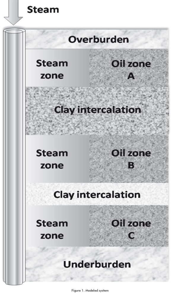
The assumptions for the development of the selected model are presented in three groups, as follows: producing zones, non-producing zones, and steamflood.

• Producing zones:  these are homogeneous formations with uniform thickness that exhibit finite thermal conductivity.
• Non-producing zones: these are represented by impermeable strata, as follows: clay intercalations and   adjacent formations to the system upper and lower limits. Despite these formations do not contribute with fluids to production, their characterization is very important since there is heat transfer to these formations from the areas submitted to steamflood.
• Clay intercalations. These are horizontal formations with uniform and finite thickness. Their horizontal thermal conductivity is zero whilst the vertical thermal conductivity is finite.
• Overburden and underburden. These formations have the same characteristics as clay intercalations. The only difference is that they are modeled as infinite thickness solids.

Steamflood.  Regarding the description of steamflood, it is defined that:

• It is conducted at a system concentric point.
• Steam enters simultaneously into all the producing zones at the same rate per unit of volume.
• A temperature vertical gradient does not exist in the producing zone.
• A noticeable drop of pressure does not exist in the steam zone.
• Heat losses are observed only in vertical direction.
• Heat transfer is negligible in front of the condensation area.

Initial condition. The initial condition for the mo-deled system is given by the temperature of producing zones, clay intercalations, and adjacent formations to the system's limits, just before the initiation of the steamflood process.

In this particular case, an average initial temperature is assumed in function of the temperature at the zones involved in the model, which are expressed as:

Boundary Conditions.  The only boundary condition for the modeled system is that during steamflood, the contacts between the steam zone and non-producing zones remain at steam temperature.

Mathematical approach

When one-layer reservoir is submitted to steamflood, it is possible to assume that the volume in the steam zone is equivalent to the volume of the heated zone. Considering that the volume of the heated zone can be determined from heat balance at the steam zone, an expression for the oil displacement rate is obtained as a function of volume variation of the steam zone. 

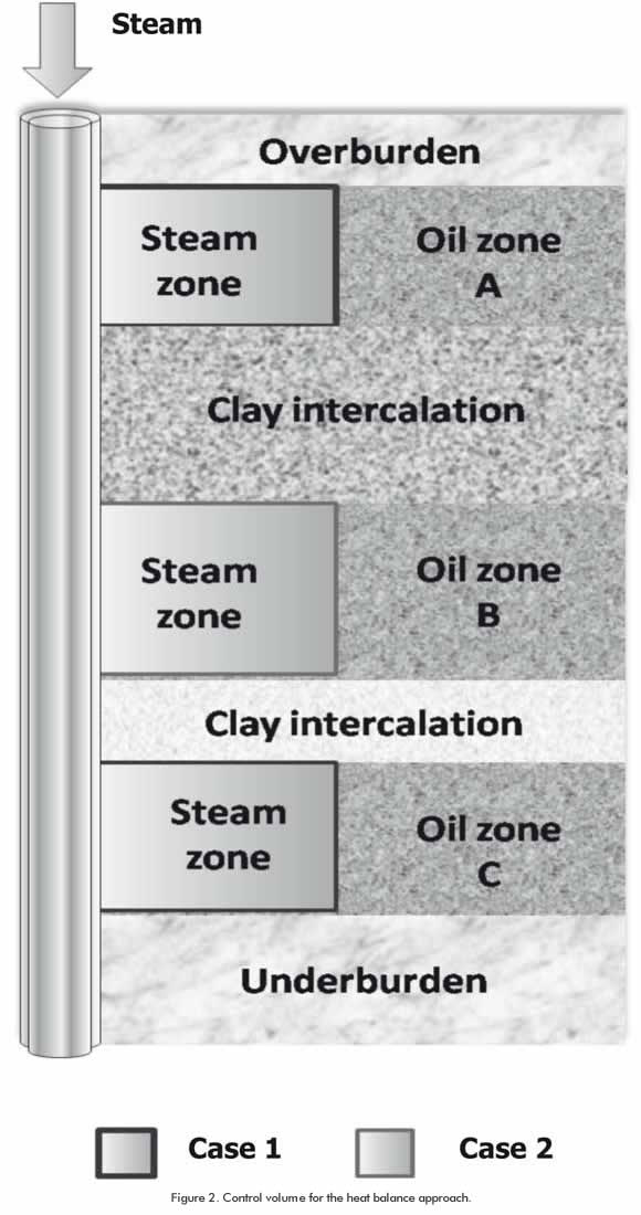
Regarding reservoirs with clay intercalations and producing zones submitted to continuous and simultaneous steamflood, modeling completion is achieved if the system is considered as a series of one-layer reservoirs. Therefore, it is necessary to propose a heat balance on each one of the steam zones present in the model, as it is illustrated in Figure 2. In general terms, two study cases are identified:

Study Case 1: the producing zone is bordered by a clay intercalation and the overburden or underburden.

Study Case 2: the steam zone is bordered by two clay intercalations.

The main difference between the balance terms proposed for the cases 1 and 2 is represented in the heat loss term. In case 1, heat losses are present toward an infinite thickness zone and toward a finite thickness zone. In case 2, heat losses shall be defined by heat flow toward two finite - thickness zones.

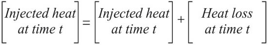
From the Law of Energy Conservation, it is stated that:

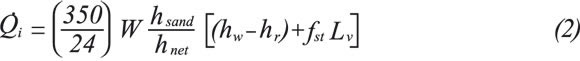
Heat injection rate in the Producing Zone.  The energy entering producing zones is represented by the heat transported by the steam being flooded. It is worth highlighting that a fraction of the total steam volume reaching the well is introduced to each producing zone, assuming that the same quantity of energy per net thickness unit enters. Therefore, the rate of energy entering the formation depends on the rate at which steam is injected, steam thermal properties, and thickness of the sand submitted to steamflood.

The heat injection rate to producing zones from the mathematical standpoint is given by:

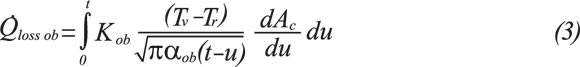
Heat Loss Rate.  In a stratified system as the one modeled, heat losses are defined by the heat transferred to the non-producing zones per unit of time. Because there is no fluid flow in non producing zones, heat transfer occurs by conduction. Therefore, heat flow is quantified from Fourier’s Law considering that overburden and underburden are of infinite thickness and clay intercalations have finite thickness.

Heat loss toward overburden and underburden is taken from the modeling completed by Marx and Langenheim (1959), as follows:

The heat loss rate toward clay intercalations is determined by a heat additional balance on a volume element belonging to this formation. For this balance, it is assumed that clay intercalations behave as a finite thickness solid in which the top and the base have the same steam temperature. The following is obtained from this approach:

Energy accumulation rate in the heated zone.  The energy accumulation rate in the heated zone represents the amount of heat employed per unit of time to take the formation together with the interstitial fluids from the reservoir temperature to the steam temperature. From the mathematical standpoint, it is given by:

Upon obtaining each term composing the heat balance, these are grouped according to the case, as follows:

Case 1:

Case 2:

Calculations for the steam zone: case 1. The following expression is obtained by replacing each heat balance term for case 1:

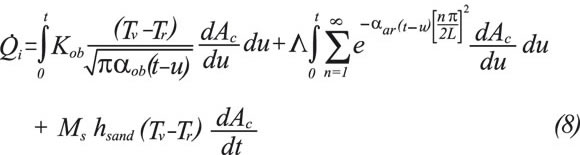
Equation 8 is solved, considering that the steam zone volume is given by the product of the heated area and the thickness of the flooded zone. Because the expression obtained is an integro-differential equation, it is necessary to employ the solution by the Laplace transform method, as follows:

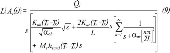
An expansion of the denominator sum is conducted  to facilitate the management of Equation 9. Therefore, the terms 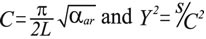are defined.

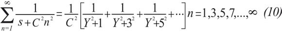
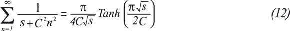
Using the formulas 949 and 950 presented by Jolley in Summation of Series (Jolley, 1961):

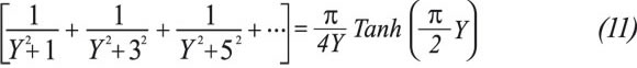
Replacing Equation 11 in Equation 10

Rewriting Equation 9, it is obtained:

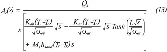
The Laplace Transforme theory establishes that it is possible to find f(t) from f(s) by the utilization of the inversed transformed calculus techniques. In this particular case, the complex inversion formula was used (Carslaw, & Jaeger, 1943; Spiegel, 1998) to obtain the heated area in function of time, from A_c(s) given in Equation 13.

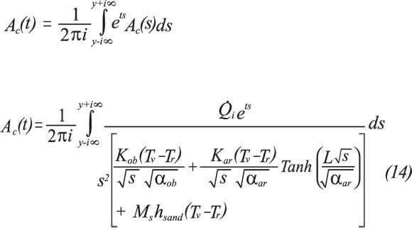
The following constants are defined to facilitate the management of Equation 14:

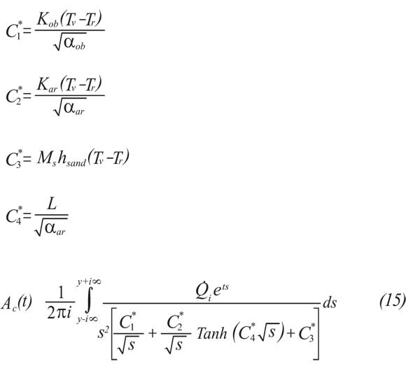
In order to solve Equation 15, it is necessary to apply the residue theorem by calculating the function poles. The function poles for Equation 15 are defined by the s values for which the nominator is zero. By conducting a superficial analysis, it is evident that s=0  behaves as a double pole and therefore the attention is focused on the calculation of additional poles.

From the expression:

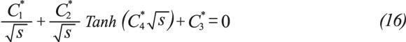
Replacing 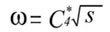in Equation 16

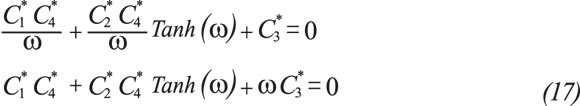
The expression 15 has infinite pole in  where ω_n are the roots of Equation 17.

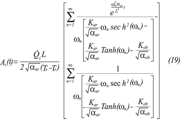
Then, the solution for the heated area as a function of time is given by:

Solving Equation 18, the area of the steam zone as function of time is obtained, considering that the heated area at time zero is zero (Mercado, Muñoz, Pérez, & Ordóñez, 2008).

The volume of the heated zone shall be equivalent to the product of the steam zone area and sand thickness.

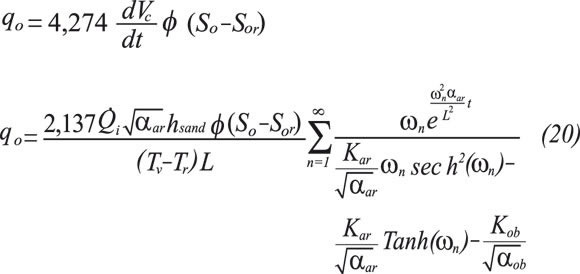
The oil displacement rate, as a result of steamflood, is given by the rate at which the mobile oil present in the steam zone is displaced. It is expressed as follows:

Cumulative heat losses in a given time, alter the initiation of steamflood and are determined from a heat balance, as follows:

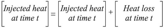
By replacing each term in the balance, it is obtained:

The instantaneous heat loss rate is expressed as follows:

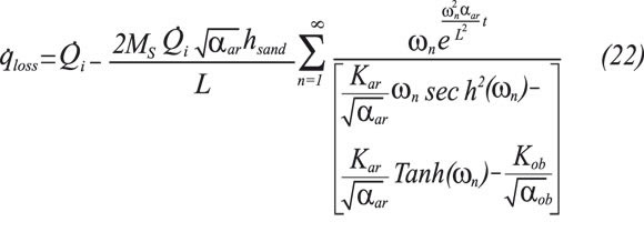
Replacing each term in the expression above:

Calculation for the Steam Zone: case 2.  Similarly to the procedure in case 1, this sections presents the calculations to determine the heated zone volume, the oil displacement rate and the cumulative and instantaneous heat loss rates when the steam zone is located between two clay intercalations.

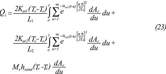
The heated zone area is calculated by replacing each term involved in the heat balance expressed in Equation 7, as follows:

Similarly to case 1, the Laplaced Transformed is obtained for each term in Equation 24.

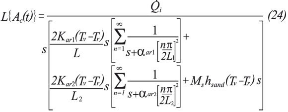
Replacing the summation equivalent of the denominator in Equation 25 by the expression presented in Equation 12, it is obtained:

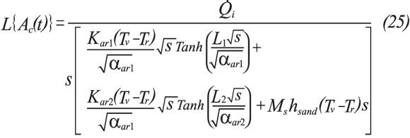
The following terms are defined to facilitated management of Equation 26:

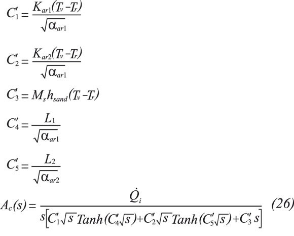
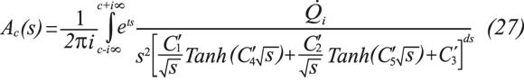
By applying the complex inversion formula, the steam heated area is given by the following equation:

A preliminary analysis of Equation 28reveals that  s = 0 behaves as a double pole. It is then necessary to focus on the determination of additional poles. From the expression:

Considering that the relation between the tangent and the hyperbolic tangent or fan angle is given by (Abramowitz & Stegun, 1968):

Replacing Equation 30 in Equation 29 and defining

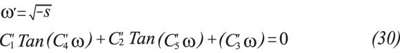
Then ω'_n are the roots of Equation 31, therefore, multiple poles are found in s = ω'²_n

Then, the solution for the heated area is given by:

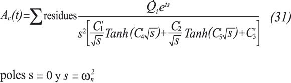
The expression for the calculation of the heated area is obtained by solving Equation 32.

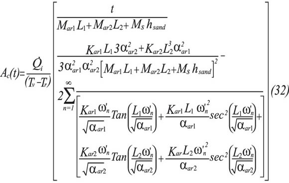
The steam zone volume is given by the product between the heated area and the thickness of the flooded area.

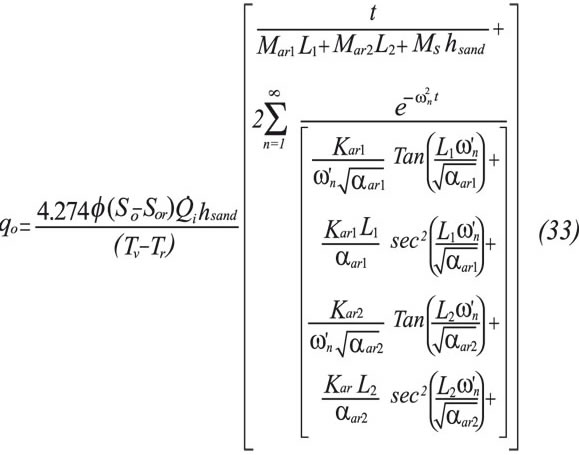
The oil displacement rate, resulting from continuous steam injection, is given by:

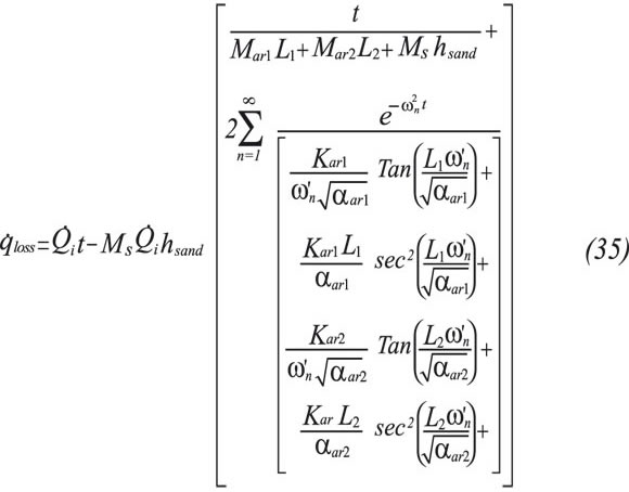
The cumulative heat loss rates are determined in the same form as in Case 1, as follows:

Finally, the instantaneous heat loss rate is expressed as:

EVALUATION OF ANALYTICAL MODEL RESULTS

The objective of designing the analytical model proposed was to predict the behavior of steamflood in stratified reservoirs. Therefore, this conceptual model of reservoir was designed (Duitama, 2005), (Salas, 2005) in order to group the main characteristics related to reservoir geology, thermal properties of rocks and fluids, fluid properties and characteristics of the rock - fluid interactions that are characteristic in a stratified reservoir intended to be submitted to steamflood.

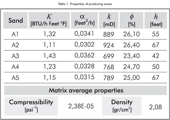
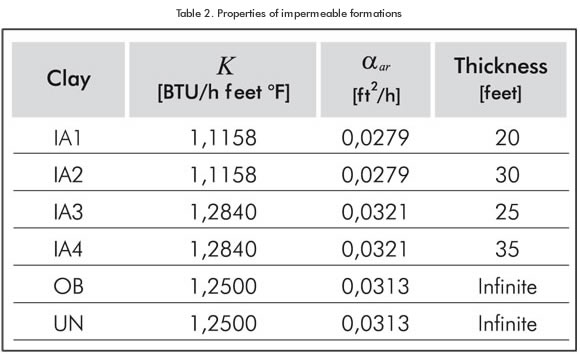
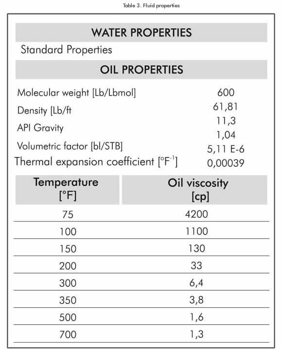
The reservoir conceptual model represents an inverse  five-point injection arrangement in a 2,5 acre area. The top of the formation is located at 1.365 feet depth, the initial average temperature is 105°F (313,70 K) and the pressure of reference is 890 psi at 1.600 feet. The reservoir is mainly composed by five producing sands and tour clay intercalations whose characteristics are summarized in Tables 1 and 2, respectively. In addition, Table 2 includes the overburden (OB) and underburden (UB) properties. The porous volume is occupied by water and oil whose characteristics are summarized in Table 3.

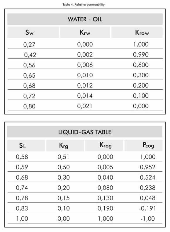
Besides the reservoir rock and fluid properties, it is necessary to establish the rock-fluid interaction. This is determined from the relative permeability curves whose values are presented in Table 4 (Basham, 2004). A 3-year steamflood is established within operational parameters, where steam is injected at a temperature of 570°F (572,038 K), a pressure value of 1.200 psi and 65 % quality in the wellbore. The injection rate has been defined to be in function of the area and thickness in a relation of 1,5 BTU / day acre feet as it is shown in Table 5.

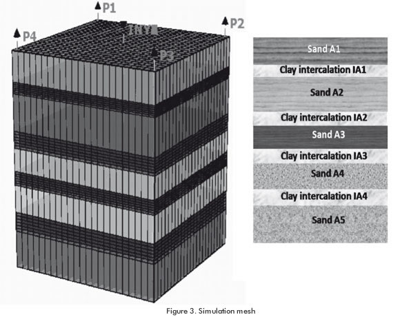
A simulation model was constructed from the conceptual model presented to evaluate the results of the analytic model.  The Steam, Thermal and Advanced Processes Reservoir Simulator (STARS) belonging to the company Computer Modeling Group (CMG) was utilized for the development of the above mentioned study.

In this particular case, a Cartesian mesh of 23*23*9 was utilized, with Cartesian refining in the K of 6 direction for layers 2, 4 and 6 representing clay (Figure 3). In addition, the fact that there is no fluid flow in clay intercalations was considered. Therefore, they were represented as thermal blocks where only heat balance calculations are conducted.

Evaluation of the results obtained for Case 1: the initial evaluation of the results obtained with the model was conducted separately for each of the cases proposed.  Considering that Case 1 represents producing zones located between the overburden or underburden and a clay intercalation, the model was evaluated for the A1 sand. Figure 4 illustrates the graph of heated area and oil recovery factor in function of time.

Since the results exhibit a physical coherence with the phenomenon intended to predict, a response comparison for A1 and A5 sands with the analytical model for Case 1 and simulation is presented.

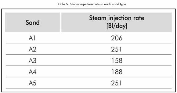
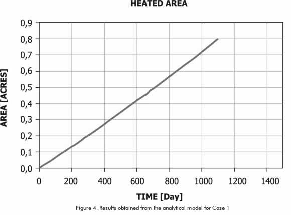
Figure 5 illustrates that the oil production rate calculated from the analytical model is below the rate predicted by numerical simulation. This subestimation of the oil production rate is due to the fact that analytical models don't consider parameters such as drop pressure, relative permeability and oil viscosity which affect the reservoir behavior.

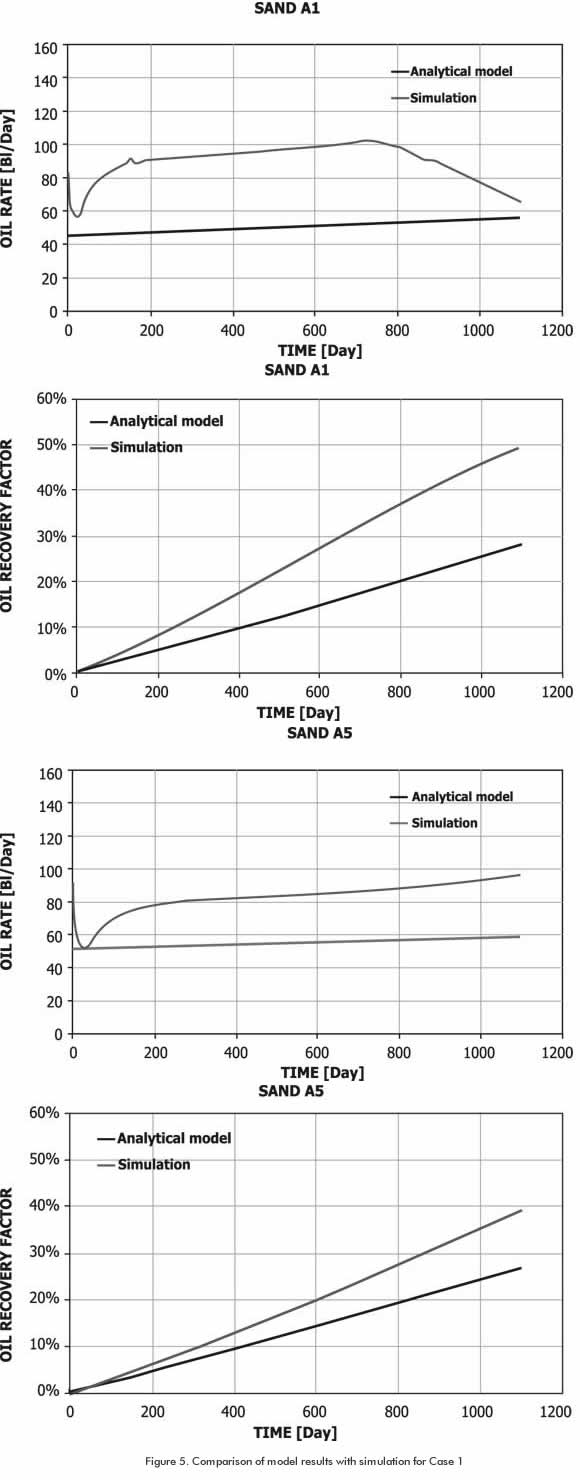
In this case we assume that there is enough pressure gradient across the formation, so fluids are produced at the predicted rate. The simulator, instead, considers the effect of this parameter from the quantitative standpoint.

The fall of the production curve predicted by the simulator for Sand A1 can be associated to steam breakthrough to producing wells. Therefore, the analytical response of analytic models must be analyzed until this point. Based on the above, the analytical model for stratified reservoir shows a tendency according to sand response. This appreciation is clearly ratified in the sand 5 case where steam breakthrough is not observed yet. Difference in breakthrough times between sands A1 and A5 is a consequence of the pressure distribution in the simulation model, whose calculation is based on sand depth. In this case the analytical model response is better when the well producer pressure is high because the drop pressure in the steam zone is not noticeable.

Result evaluation for Case 2.  The evaluation of the analytical model proposed for Case 2 was conducted separately for A2, A3 and A4 sands, considering that these sands are located between two clay intercalations. Initially, an evaluation was conducted for sand A3 and the results are shown in Figure 6.

Case 2 results are physically coherent with the response that sand A3 might have to steamflood, as it can be implied from Figure 6. Therefore, a comparison with numerical simulation is conducted.

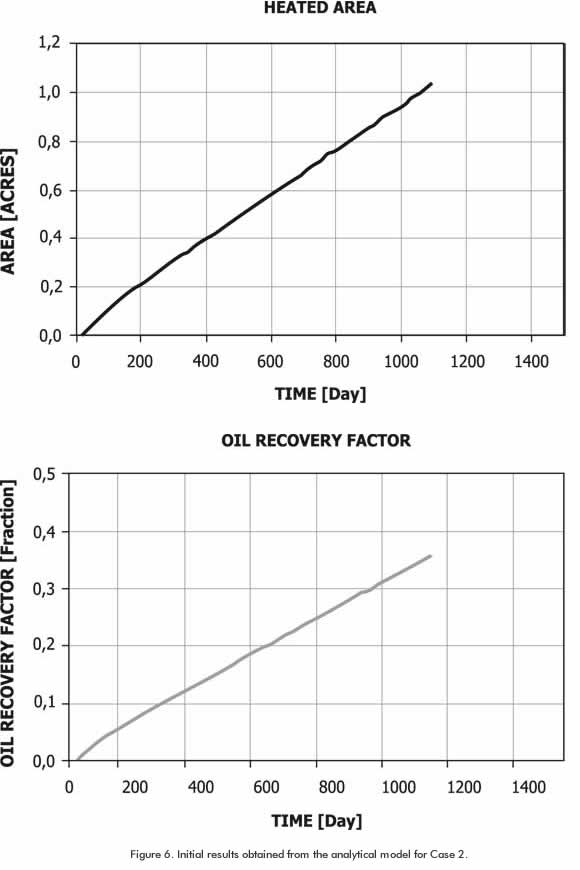
Figure 7 shows that the model proposed represents the acceptable behavior of steamflood in sands located between two clay intercalations.

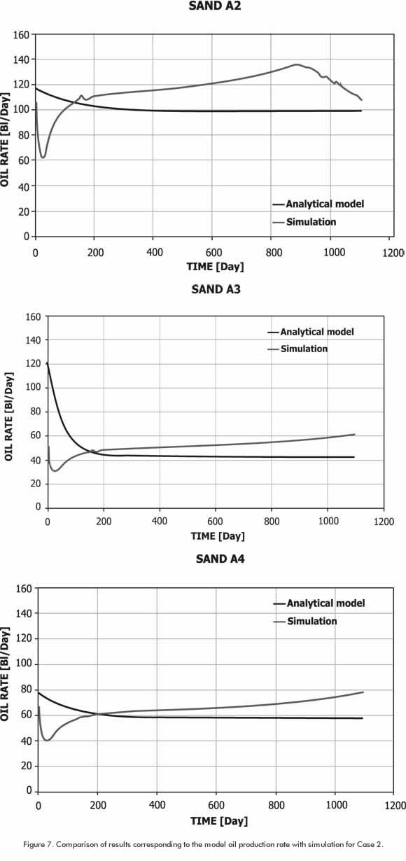
The response presents a greater tendency compared to the trend obtained by simulation as intercalation thickness increases. This is due to the assumption on which the model is developed, that established the existence of a heat flow in non-stationary state in this formation during the injection process.

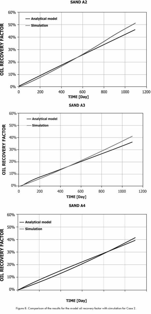
Taking the oil recovery factor presented in Figure 8 as reference, the model describes the behavior of such parameter in an acceptable manner. The fact that the model response is under the simulated response is due to the fact that the simulator allows the representation of certain phenomena that could not be mathematically included in the modeling. Drop pressure across the formation, the effect of pressure on steam properties, steam condensation, and rock-fluid interaction are among these phenomena.

Although the model does not consider the above mentioned phenomena, it can be described heat flow toward impermeable formation in more detail. Therefore, it is a valuable tool to determine heat requirement in the project. It is worth mentioning that the parameters compared were selected considering that each tool allows the visualization of such results.

CONCLUSIONS

• Heat flow quantitative analysis through each element composing a stratified reservoir allows the structuring of models that predict the behavior of steamflood in a more approximate manner.
• The fact that the proposed analytical model describes the tendency of the oil production rate by numerical simulation leads to the indirect conclusion that this is a reliable model for the evaluation of parameters such as growth of steam zone with time, and cumulative and instantaneous heat losses produced during the injection.
• The proposed analytical model describes the behavior of parameters such as heated area, oil production rate, heat loss, and oil recovery factor in heavy crude oil stratified reservoirs in a more approximate manner. In these cases, a heat flow in a non-stationary state through clay is maintained.

ACKNOWLEDGMENTS

The authors express their feelings of gratitude to the Enhanced Oil Recovery Group at Universidad Industrial de Santander (UIS), and to Dr. S. M. Farouq Ali for his orientation and interest during the development of this work.

REFERENCES

Abramowitz, M. & Stegun, I. ( 1968). Handbook of mathematical tables. USA (55): National bureau of standards applied mathematics series. 64-60036.        [ Links ]

Basham, M. (2004). Important modeling parameters for predicting steamflood performance. SPE 90713.         [ Links ]

Carslaw, H. S. & Jaeger, J. C. (1943). Operational methods in applied mathematics. Great Britain : Oxford University Press.          [ Links ]

Closmann, P. J. (1967). Steam zone growth during multiple-layer steam injection. SPE 1716.          [ Links ]

Duitama, J. (2005). Estandarización de los procedimientos de perforación en los pozos del campo Jazmín. Tesis de grado Facultad de Ingeniería de Petróleos, Universidad Industrial de Santander, Bucaramanga, Colombia.        [ Links ]

Jolley, L. B. (1961). Summation of series. New York: Dover Publications.        [ Links ]

Mandl, G. & Volek, C. W. . (1967). Heat and mass transport in steam-drive processes. SPE 1896.         [ Links ]

Marx, J. W. & Langenheim, R. H. (1959). Reservoir heating by hot fluid injection. SPE 1266-G.         [ Links ]

Mercado, D., Muñoz, S., Pérez, H. & Ordóñez, A. (2008). Modelo analítico para predecir el comportamiento de la inyección continua de vapor en yacimientos estratificados de crudo pesado. Trabajo de investigación. Magíster en Ingeniería de Hidrocarburos. Universidad Industrial de Santander. Bucaramanga. Colombia.        [ Links ]

Salas, A. (2005). Análisis de las operaciones de cementación, empaquetamiento con grava y los fluidos de perforación para un pozo tipo en el caso Jazmín. Tesis de grado Facultad de Ingeniería de Petróleos, Universidad Industrial de Santander, Bucaramanga, Colombia.        [ Links ]

Spiegel, M. (1998). Transformadas de Laplace. México: McGraw-Hill.        [ Links ]