ABSTRACT

It is expected for naturally occurring formations that the transition period of flow from fissures to matrix takes place during the radial flow regime. However, depending upon the value of the interporosity flow parameter, this transition period can show up before or after the radial flow regime. First, in a heterogeneous formation which has been subjected to a hydraulic fracturing treatment, the transition period can interrupt either the bilinear or linear flow regime. Once the fluid inside the hydraulic fracture has been depleted, the natural fracture network will provide the necessary flux to the hydraulic fracture. Second, in an elongated formation, for interporosity flow parameters approximated lower than 1x10^-6, the transition period takes place during the formation linear flow period. It is desirable, not only to appropriately identify these types of systems but also to complement the conventional analysis with the adequate expressions, to characterize such formations for a more comprehensive reservoir/well management.

So far, the conventional methodology does not account for the equations for interpretation of pressure tests under the above two mentioned conditions. Currently, an interpretation study can only be achieved by non-linear regression analysis (simulation) which is obviously related to non-unique solutions especially when estimating reservoir limits and the naturally fractured parameters. Therefore, in this paper, we provide and verify  the necessary mathematical expressions for interpretation of a vertical well test in both a hydraulically-fractured naturally fractured formation or an elongated closed heterogeneous reservoir. The equations presented in this paper could provide good initial guesses for the parameters to be used in a general nonlinear regression analysis procedure so that the non-uniqueness problem associated with nonlinear regression may be improved.

Keywords: Dual-linear flow regime, radial flow regime, interporosity flow parameter, dimensionless storativity ratio

RESUMEN

Se espera en formaciones naturalmente fracturadas que el periodo de transición de las  fisuras a la matriz tome lugar durante el flujo radial. Sin embargo, dependiendo del valor del parámetro de flujo interporoso, esta transición puede ocurrir antes o después del flujo radial. El primer caso, en una formación heterogénea que ha sido sometida a un tratamiento de fracturamiento hidráulico, la transición puede interrumpir el flujo bilineal o lineal tempranos. Una vez existe depleción de flujo en la fractura hidráulica, éste es restablecido por flujo procedente de la red de fracturas naturales. En el segundo escenario, en una formación alargada, para parámetros de flujo aproximadamente menores a 1x10^-6, el periodo de transición ocurre durante el flujo lineal en la formación.  Se desea no solo identificar estos sistemas apropiadamente sino complementar la técnica convencional con las expresiones adecuadas para caracterizar tales formaciones de modo que se tenga un manejo más comprensivo del yacimiento/pozo.

Hasta ahora, la técnica convencional no cuenta con las ecuaciones para interpretar pruebas de presión bajo las dos condiciones arriba descritas. Actualmente, la única forma de interpretación se conduce mediante técnicas de regresión no lineal (simulación) lo que conlleva a problemas de múltiples respuestas especialmente cuando se estiman los límites del yacimiento y los parámetros del yacimiento naturalmente fracturado. Por tanto, en este artículo, se proporcionan y verifican las expresiones matemáticas necesarias para interpretar pruebas de presión en un pozo vertical tanto en sistemas naturalmente fracturados interceptados por una fractura hidráulica, como en formaciones heterogéneas alargadas. Las ecuaciones presentadas en este artículo podrían proporcionar valores iniciales más representativos de los parámetros usados en un procedimiento general de regresión no lineal, de modo que se puedan reducir los problemas de multiplicidad de soluciones asociadas con este método.

Palabras Clave: Régimen de flujo dual lineal, régimen flujo radial, parámetro de flujo interporoso, coeficiente de almacenaje adimensionales

RESUMEN

Esperase em formações naturalmente fraturadas que o período de transição das  fissuras à matriz tome lugar durante o fluxo radial. Entretanto, dependendo do valor do parâmetro de fluxo interporoso, esta transição pode ocorrer antes ou depois do fluxo radial. O primeiro caso, em uma formação heterogénea que foi submetida a um tratamento de fraturamento hidráulico, a transição pode interromper o fluxo bilineal ou lineal precoces. Uma vez exista depleção de fluxo na fratura hidráulica, este é reestabelecido por fluxo procedente da rede de fraturas naturais. No segundo cenário, em uma formação alongada, para parâmetros de fluxo aproximadamente menores a 1x10^-6, o período de transição ocorre durante o fluxo lineal na formação.  Caso deseje não somente identificar estes sistemas apropriadamente senão complementar a técnica convencional com as expressões adequadas para caracterizar tais formações de modo que se tenha um manejo mais compreensivo da jazida/poço.

Até agora, a técnica convencional não conta com as equações para interpretar provas de pressão sob as duas condições encima descritas. Atualmente, a única forma de interpretação é conduzida mediante técnicas de regressão não lineal (simulação) o que tem como consequéncias a problemas de múltiplas respostas especialmente quando se estimam os limites da jazida e os parâmetros da jazida naturalmente fraturada. Portanto, neste artigo, se proporcionam e verificam as expressões matemáticas necessárias para interpretar provas de pressão em um poço vertical tanto em sistemas naturalmente fraturados interceptados por uma fratura hidráulica, como em formações heterogéneas alongadas. As equações apresentadas neste artigo poderiam proporcionar valores iniciais mais representativos dos parâmetros usados em um procedimento geral de regressão não lineal, de modo que se possam reduzir os problemas de multiplicidade de soluções associadas com este método.

Palavras Chave: Regime de fluxo dual lineal, regime fluxo radial, parâmetro de fluxo inter-poroso, coeficiente de armazenagem adimensionais

NOMENCLATURE

4n(n+2)12 = Slab model, 32 = Matchstick model, 60 cubic model

A     Area, (ft2)

B     Oil formation factor, (rb/STB)

C_fD   Dimensionless fracture conductivity

c_t     Compressibility, (1/psi)

h      Formation thickness, (ft)

h_m    Matrix block height, (ft)

k_f     Fracture bulk permeability, (md)

k_fb    Matrix permeability, (md)

k_f w_f  Fracture conductivity, (md-ft)

m     Slope

P      Pressure, (psi)

P_D    Dimensionless pressure

P_i    Initial reservoir pressure, (psi)

P_wf    Well flowing pressure, (psi)

P_ws   Well static pressure, (psi)

q     Flow rate, (bbl/D)

r_w     Well radius, (ft)

s_DL   Geometric skin factor due to the convergence of radial to dual-linear flow

s_L     Geometric skin factor due to the convergence of dual-linear to single-linear flow

s_r     Mechanical skin factor

T     Time, (hr)

t_D     Dimensionless time

t_DA    Dimensionless time based on reservoir area

t_Dxf   Dimensionless time based on half-fracture length

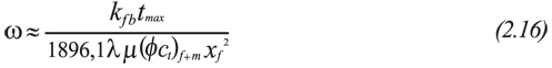
t_max  Time corresponding to the maximum pressure derivative of the transition period during either bilinear or linear flow regime, (hr)

t_min   Time corresponding to the minimum pressure derivative of the transition period, (hr)

x_f     Half-fracture length, (ft)

Y_E    Reservoir width, (ft)

W_D   Dimensionless reservoir width, (ft)

GREEK

Δ      Change, drop

Δt     Flow time, (hr)

ΔP_1hr  Pressure drop read at t  = 1 hr, (psi)

Ø     Porosity, fraction

μ      Viscosity, (cp)

λ      Interporosity flow parameter between matrix and fissures

λf     Interporosity flow parameter between hydraulic fracture and

       fissures

ω      Dimensionless storativity (capacity) ratio

SUFFICES

BL     Bilinear flow

D      Dimensionless

DA    Dimensionless referred to reservoir area

DLF   Dual-linear flow

f       Fracture network, fissures

f+m  Total system (fracture network + matrix)

i       Initial conditions

L      Single-linear flow

LF     Single-linear flow

m     Matrix, slope

max  Maximum

min   Minimum

INTRODUCTION

Recently, Tiab and Bettam (2007) have introduced a technique to interpret pressure and pressure derivative tests in heterogeneous formations drained by a hydraulically fractured vertical well. Also, we are aware that an important number of pressure tests are conducted in long and narrow reservoirs which may possess heterogeneous nature with very low mass transfer capacity between fracture network and matrix. In the first case, the transition period may take place before the radial flow is developed. Once the flux in the hydraulic fractured is depleted, the naturally occurring fractures fed the hydraulic fracture, allowing the development of the transition period. In the second case, the phenomenon occurs after radial flow is vanished. During either dual-linear or linear flow  regime in the formation, the fracture network fluid is depleted and, then, being reestablished from the matrix, leads to the presence of the transition period. In both cases, this transition period takes a "V" shape on the pressure derivative curve.

Among the investigations on pressure tests for elongated systems during this decade, Escobar et al. (2007a) introduced the application of the TDS technique for characterization of long and homogeneous reservoirs presenting new equations for estimation of reservoir area, reservoir width and geometric skin factors. Characterization of pressure tests in elongated systems using the conventional method was presented by Escobar and Montealegre (2007). Also, Escobar et al. (2007b) provided a way to estimate reservoir anisotropy when reservoir width is known in the mentioned systems from the combination of information obtained from the linear and radial flow regimes.

In this work, new expressions to complement the conventional technique are presented for interpretation of pressure tests in naturally occurring formations when the transition period takes place either before of after the radial flow regime. The proposed equations were verified with several examples.

MATHEMATICAL MODEL

The main assumptions considered in this work are: a slightly compressible and constant viscosity fluid flows throughout a constant thickness reservoir with constant matrix and fracture permeability and porosity, the well fully penetrates the producing formation. Flow from the natural fracture network to either hydraulic fracture or matrix occurs under pseudosteady state conditions. Neither wellbore storage nor geomechanical skin factor nor gravity effects are considered.

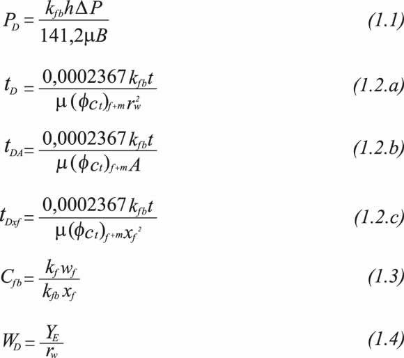
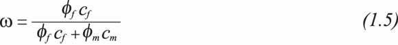
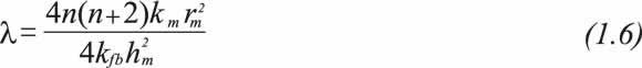
The dimensionless quantities are defined as:

The naturally fractured reservoir parameters, dimensionless storativity (capacity) ratio and interporosity flow, introduced by Warren and Root (1963) were defined by:

THE TRANSITION PERIOD OCCURS BEFORE RADIAL FLOW REGIME

According to Tiab and Bettam (2007) the bilinear flow regime of a finite-conductivity hydraulic fracture in a heterogeneous formation is governed by:

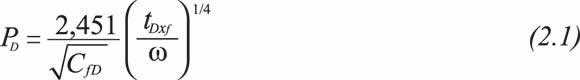
Substituting the dimensionless quantities, Equations. 1.1, 1.2.c and 1.3 into Equation 2.1, yields:

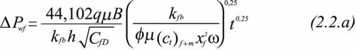
For pressure buildup analysis, application of time superposition is required, therefore Equation 2.2.a becomes:

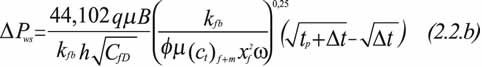
The above expressions imply that a Cartesian plot of DP vs. either t^0,25 or [(t_p+Dt)^0,25- Dt^0,25] will yield a straight line with slope, m_BL:

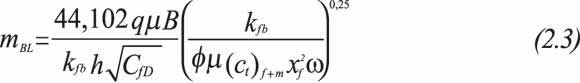
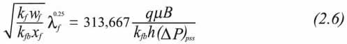
Solving for the fracture conductivity, k_fw_f, results:

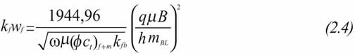
Figure 1 is a plot of P_DC_fD^0,5λ_f^0,25 versus λt_Dxf/w. It is observed there that during the pseudosteady state transition period P_Dλ_f^0,5 yields a horizontal line defined by Tiab and Bettam (2007) as:

Replacing Equations 1.1 and 1.3 into Equation 2.5 and solving for λ_f  yields:

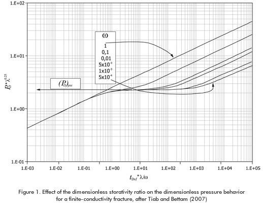
It is observed for the first bilinear flow regime that the curves for the same interporosity flow parameter coincide for different values of dimensionless capacity ratio. See Figure 1. A correlation for this line yields:

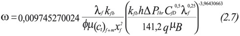
Equation 2.7 has a correlation coefficient of 0,99994583 and should be valid for ω ≥ 0,005.

Also, according to Tiab and Bettam (2007), the linear flow regime during early time is governed by:

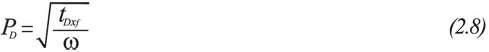
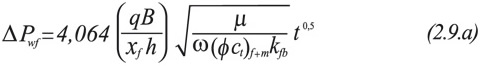
Substituting in Equation 2.8 the dimensionless quantities, Equations 1.1 and 1.2.c, respectively, yields:

Application of time superposition to Equation 2.9.a leads to:

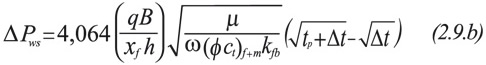
Equations 2.9.a and 2.9.b imply that a Cartesian plot of ΔP vs. either t ^0,5 or [(t_p+Δt)^0,5- Δt ^0,5] will yield a straight line with slope, m_L:

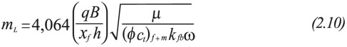
Solving for the fracture conductivity, x_f, results:

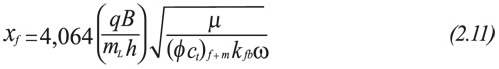
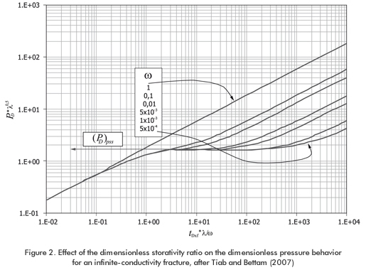
Figure 2 is a plot of P_Dλ_f ^0,5 versus λ_f t_Dxf /w. As pointed out by Tiab and Bettam (2007), it is observed that during the pseudosteady state transition period P_Dλ_f ^0,5 is a horizontal line:

Substituting for the dimensionless term, Equation 1.1, and solving for λ_f results:

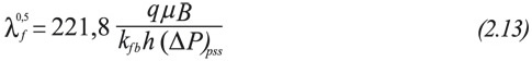
Notice that for the first linear flow, the lines for the same interporosity flow parameter coincide for different values of storativity coefficient ratio. A correlation for this line yields:

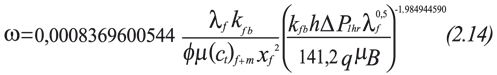
Equation 2.14 has a correlation coefficient of 0,999971228 and should be valid for ω≥ 0,005.

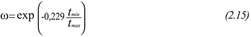
Finally, Tiab and Bettam (2007) found that the pressure derivative displays a maximum pressure once the transition period begins, and a minimum point during the transition period. If these points are feasible of being obtained, the dimensionless storativity ratio can be estimated for bilinear and linear flow regime, respectively, by:

THE TRANSITION PERIOD OCCURS AFTER RADIAL FLOW REGIME

In elongated reservoirs where the mass transfer between matrix and fractures is delayed due to very low interporosity flow parameters, less than 1x10^-7, the transition period takes places once radial flow regime has vanished. Either dual-linear or single-linear flow regime may be interrupted by the transition period in which the fracture network is fed by the matrix. For the case of transient rate analysis, this behavior may show up during the late pseudosteady state period, though.

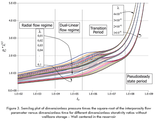
Figure 3 displays a semilog plot of the dimensionless pressure, times the square-root of the interporosity flow parameter versus dimensionless time for different dimensionless capacity ratios. This plot can provide better detail than the pure dimensionless pressure plots. As expected, an early linear trend is observed indicating the infinite transient behavior. Afterwards, the dual- linear flow regime appears. However, part of it is obscured by the radial flow regime. During the late pseudosteady state period, all the lines for different dimensionless storativity ratios coincide for each interporosity flow parameter.

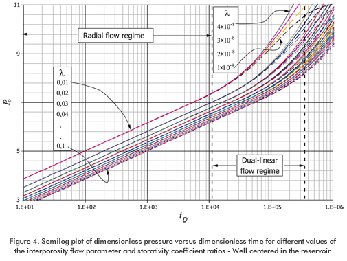
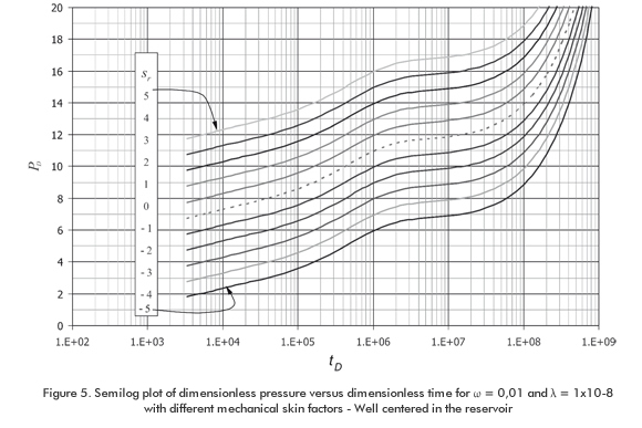
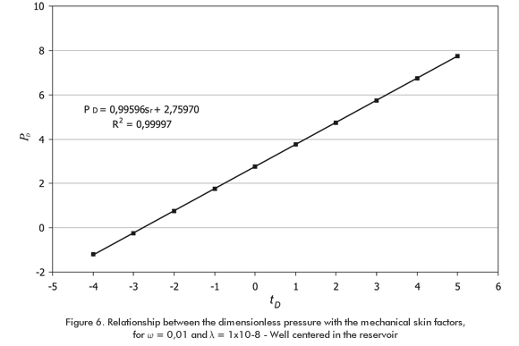
Figure 4 is a semilog plot of the dimensionless pressure versus dimensionless time for different values of the interporosity flow parameter and storativity coefficient ratios. Part of the transition period is shown in the plot. It is observed that the lines for the same storativity coefficient ratio coincide for the same value of the interporosity flow parameter. A correlation between ω and the intercept of the semilog plot has a correlation coefficient of 0,99999872 and a standard deviation of 3,2973259x10^-5. The range of application of this correlation is 0,01≤ ω ≤ 0,1 and -5 ≤ s_r  ≤ 5. This is given below as:

As shown in Figure 5, the intercept of the semilog plot is a direct function of the skin factor. The correlation between skin factor and the intercept is shown in Figure 6. Equation 3.1 already includes this effect.

The interporosity flow parameter can be approximated by the equation provided by Tiab and Escobar (2003):

The Transition Period Occurs During The Dual-Linear Flow Regime

Escobar et al. (2009) presented the governing equation for dual-linear flow regime in a naturally fractured reservoir:

After replacing the dimensionless quantities in the above expression, it yields:

For pressure buildup analysis, application of time superposition is required, therefore Equation 3.4 becomes:

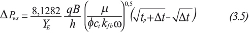
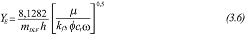
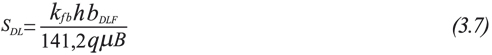
Equations 3.4 and 3.5 indicate that a Cartesian plot of ΔP vs. either t0,5 or [(tp+Δt)0,5- Δt0,5] will yield a straight line during dual-linear flow behavior which slope, mDLF, and intercept, bDLF, are used to obtain reservoir width, YE, once the storativity coefficient ratio is determined and dual-linear skin factor, sDL.

Linear-Flow Regime Occurs After The Transition Period

Once the transition period disappears, the reservoir behaves as homogeneous; then, the single-linear flow regime appears, which governing equations for pressure and pressure derivative presented by Escobar et al. (2007a) and Escobar and Montealegre (2007) are:

Replacing Equations 1.1, 1.2.a and 1.4 into the above expression results:

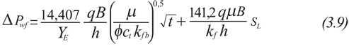
and for buildup pressure tests Equation 3.9 becomes:

This implies that a Cartesian plot of ΔP vs. either t 0,5 or [(tp+Δt) 0,5- Δt 0,5] will yield a straight line during duallinear flow behavior which slope, mLF, and intercept, bLF, are used to obtain reservoir width, YE, once the storativity coefficient ratio is determined and linear skin factor, SL.

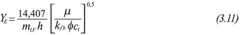
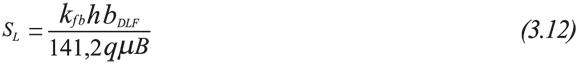
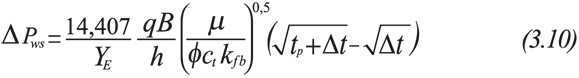
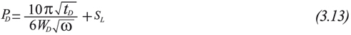
Linear-Flow Regime Occurs Before The Transition Period

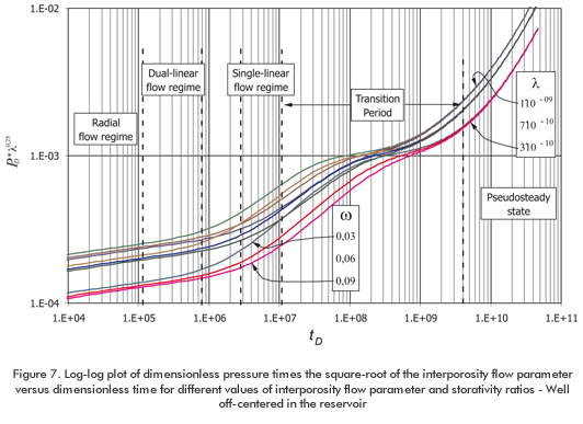
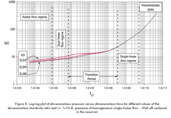
According to Escobar et al. (2009), this case, which is described by Figures 7 and 8, has the following governing equation:

Once the dimensionless quantities are replaced in Equation 3.13, the following expression is obtained:

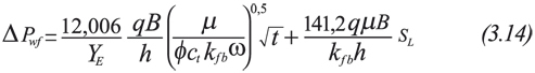
For pressure buildup analysis, application of time superposition is required, therefore Equation 3.14 becomes:

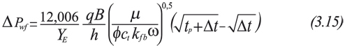
This implies that a Cartesian plot of ΔP vs. either t 0,5 or [(tp+Δt)0,5- Δt0,5] will yield a straight line during linear flow behavior which slope, mLF, and intercept, bLF, are used to obtain reservoir width, YE, once the storativity coefficient ratio is determined and single-linear skin factor, SL.

EXAMPLES

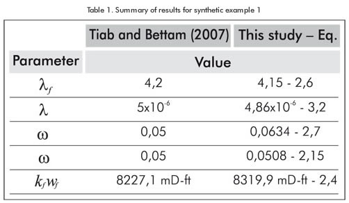
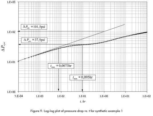
Synthetic Example 1

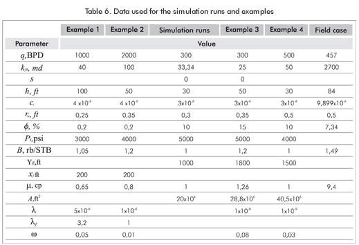
A synthetic pressure test for a well in an infinite reservoir was generated by Tiab and Bettam (2007) with information from Table 1. Characterize this hypothetic reservoir using conventional analysis.

Solution

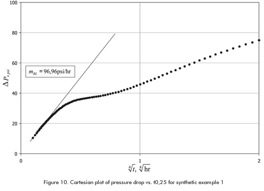
In this example the bilinear flow regime occurs before the transition period. From Figure 9, we read a value of ΔP_1hr = 101,5 psi, t_min = 0,095 hr,  t_max =  0,0073 hr, and ΔP_pss = 37,5 psi. Values of m_BL = 96,96 psi/hr are read from Figure 10. The calculations are summarized below:

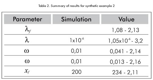
Synthetic Example 2

A simulated pressure test for a well in an infinite reservoir was generated for this work with information from Table 1. Use conventional analysis to interpret this well pressure test.

Solution

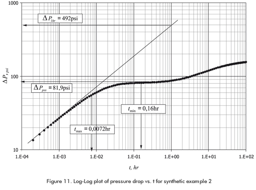
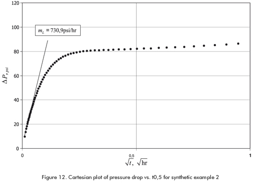
In this example the linear flow regime occurs before the transition period. From Figure 11, we read a value of ΔP_1hr = 492,0 psi,  t_max =  0,0072 hr and ΔP_pss = 82,0 psi. Values of m_L =730,9 psi/hr are read from Figure 12. A summary of results is given below:

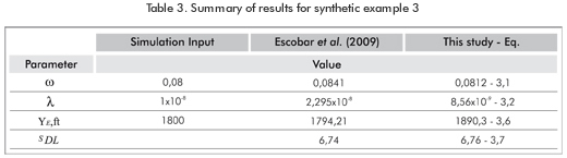
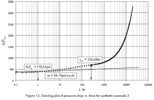
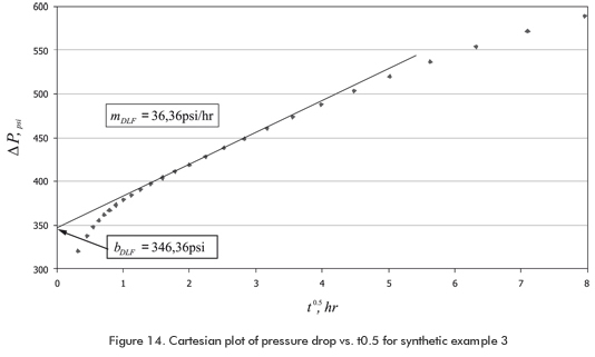
Synthetic Example 3

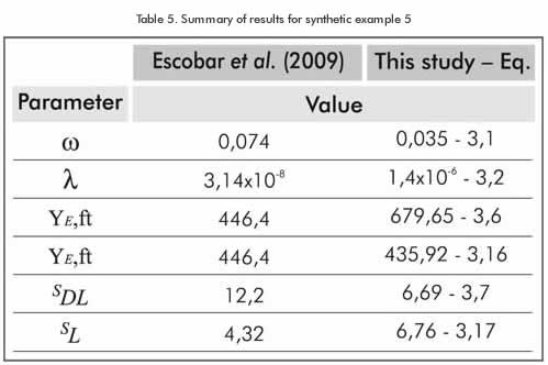
The semilog plot of a simulated drawdown generated with the information of Table 1, presented by Escobar et al. (2009) is reported in Figure 13. Characterize this hypothetic reservoir using conventional analysis.

Solution

From Figure 13, ΔP1hr = 378,81 psi is read. Values of m_DLF = 36,36 psi/hr and b_DLF = 346,36 psi are read from Figure 14. The computations are summarized and reported as follows:

Synthetic Example 4

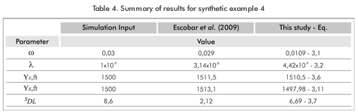
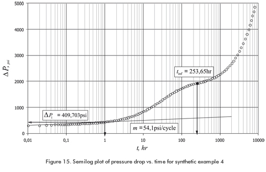
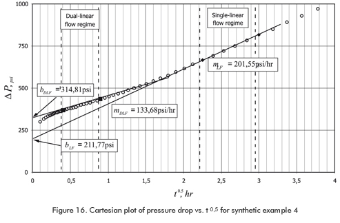
A synthetic pressure test for a well off-centered in a reservoir was also generated by Escobar et al. (2009) with information from Table 1. The pressure and pressure derivative plot is provided in Figure 15. It is required to estimate the geometric skin factors, reservoir width and the naturally fractured reservoir parameters.

Solution

From Figure 15, it is read a value of ΔP1hr = 409,703 psi. Values of m_DLF =  133,68 psi/hr, b_DLF =  314,81, m_LF = 201,55 psi/hr and  b_LF =  211,77 psi are read from Figure 16. The computations are summarized and reported as follows:

Field Example

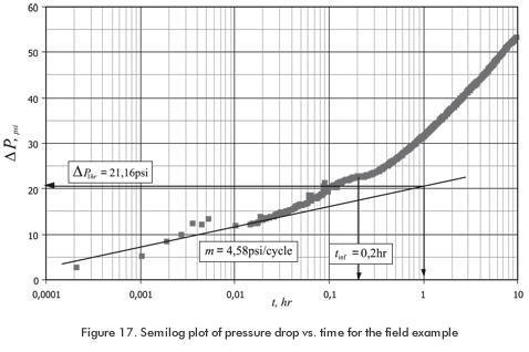
Escobar et al. (2009) also reported an example taken from a pressure test run in a South American well. Reservoir, fluid and well parameters are provided in Table 1 and the pressure data is provided in Figure 17. The reservoir permeability of 2700 md was obtained from a previous test. Find reservoir width, geometric skin factor, interporosity flow parameter and the dimensionless storativity coefficient.

Solution

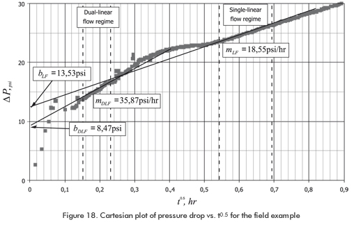
In this example the single-linear flow regime occurs after the transition period. Since permeability is known, the semilog slope can be found from the classical conventional equation giving a value of 4,58 psi/cycle. Then, ΔP_1hr = 21,16 psi is obtained using any point on the radial flow regime straight line from Figure 17. Values of m_DLF =  35,87 psi/hr,  b_DLF = 8,47, m_LF = 18,55 psi/hr and  b_LF = 13,53 psi are read from Figure 18. The computations are summarized and reported as follows:

COMMENTS ON THE RESULTS

The synthetic examples are shown to verify the introduced equations for the conventional technique. A good agreement is observed between the results obtained in this study and those from the simulation input or other sources. However, the results of the field example showed disagreement to some extent, probably due to the noisy data, as well as the accuracy of the correlations.

CONCLUSION

• New equations for the classical conventional method are introduced to characterize oil bearing heterogeneous formation when the transition period takes place outside the radial flow regime. The equation provided by Tiab and Escobar (2003) to determine the interporosity flow parameter, initially developed for transition period during the radial flow regime, has been found to provide good results for heterogeneous formations when the transition period takes place before or after the radial flow regime.

ACKNOWLEDGMENTS

The authors gratefully acknowledge the financial support of Universidad Surcolombiana for the completion of this study.

REFERENCES

Escobar, F. H., Hernandez,D.P.&Saavedra, J. A. (2009). Pressure and pressure derivative analysis for long naturally fractured  reservoirs using the tds technique. Article sent to the Dyna Journal to request publication.        [ Links ]

Escobar, F. H., Hernández, Y. A. & Hernández, C. M. (2007)a. Pressure transient analysis for long homogeneous reservoirs using tds technique. J. of Petroleum Science and Engineering, 58 (1-2), 68-82.         [ Links ]

Escobar, F. H. & Montealegre, M. (2007). A complementary conventional analysis for channelized reservoirs. CTYF- Ciencia, Tecnología y Futuro. 3(3), 137-146.        [ Links ]

Escobar, F. H., Tiab, D. & Tovar, L.V. (2007).  Determination of areal anisotropy from a single vertical pressure test and geological data in elongated reservoirs. J. of Engineering and Applied Sciences,   2(11), 1627-1639.        [ Links ]

Tiab, D. & Escobar, F. H. (2003). Determinación del parámetro de flujo interporoso a partir de un gráfico semilogarítmico. X Congreso Colombiano del Petróleo (Colombian Petroleum Symposium). Bogotá, Colombia.        [ Links ]

Tiab, D. & Bettam, Y. (2007). Practical interpretation of pressure tests of hydraulically fractured wells in a naturally fractured reservoir. Paper SPE 107013 presented at theSPE Latin American and Caribbean Petreoleum Engineering Conference held in Buenos Aires, Argentina.         [ Links ]

Warren, J. E. & Root, P. J. (1963). The behavior of naturally fractured reservoirs. Soc. Pet. Eng. Journal, September edition, 245-255.        [ Links ]